Characterizations of the exponential function

Characterization 1

The error of the product limit expression is described by:$${\displaystyle \left(1+{\frac {x}{n}}\right)^{n}=e^{x}\left(1-{\frac {x^{2}}{2n}}+{\frac {x^{3}(8+3x)}{24n^{2}}}+\cdots \right),}$$ where the polynomial's degree (in x) in the term with denominator n^k is 2k.

Characterization 2

Since $${\displaystyle \lim _{n\to \infty }\left|{\frac {x^{n+1}/(n+1)!}{x^{n}/n!}}\right|=\lim _{n\to \infty }\left|{\frac {x}{n+1}}\right|=0<1.}$$ it follows from the ratio test that ${\textstyle \sum _{n=0}^{\infty }{\frac {x^{n}}{n!}}}$ converges for all x.

Characterization 3

Since the integrand is an integrable function of t, the integral expression is well-defined. It must be shown that the function from ${\displaystyle \mathbb {R} ^{+}}$ to ${\displaystyle \mathbb {R} }$ defined by $${\displaystyle x\mapsto \int _{1}^{x}{\frac {dt}{t}}}$$ is a bijection. Since 1/t is positive for positive t, this function is strictly increasing, hence injective. If the two integrals $${\displaystyle {\begin{aligned}\int _{1}^{\infty }{\frac {dt}{t}}&=\infty \\[8pt]\int _{1}^{0}{\frac {dt}{t}}&=-\infty \end{aligned}}}$$ hold, then it is surjective as well. Indeed, these integrals do hold; they follow from the integral test and the divergence of the harmonic series.

Characterization 6

The definition depends on the unique positive real number ${\displaystyle a=e}$ satisfying: $${\displaystyle \lim _{h\to 0}{\frac {a^{h}-1}{h}}=1.}$$This limit can be shown to exist for any ${\displaystyle a}$, and it defines a continuous increasing function ${\displaystyle f(a)=\ln(a)}$ with ${\displaystyle f(1)=0}$ and ${\displaystyle \lim _{a\to \infty }f(a)=\infty }$, so the Intermediate value theorem guarantees the existence of such a value ${\displaystyle a=e}$.

Characterization 1 ⇔ characterization 2

The following argument is adapted from Rudin, theorem 3.31, p. 63–65.

Let ${\displaystyle x\geq 0}$ be a fixed non-negative real number. Define $${\displaystyle t_{n}=\left(1+{\frac {x}{n}}\right)^{n},\qquad s_{n}=\sum _{k=0}^{n}{\frac {x^{k}}{k!}},\qquad e^{x}=\lim _{n\to \infty }s_{n}.}$$

By the binomial theorem, $${\displaystyle {\begin{aligned}t_{n}&=\sum _{k=0}^{n}{n \choose k}{\frac {x^{k}}{n^{k}}}=1+x+\sum _{k=2}^{n}{\frac {n(n-1)(n-2)\cdots (n-(k-1))x^{k}}{k!\,n^{k}}}\\[8pt]&=1+x+{\frac {x^{2}}{2!}}\left(1-{\frac {1}{n}}\right)+{\frac {x^{3}}{3!}}\left(1-{\frac {1}{n}}\right)\left(1-{\frac {2}{n}}\right)+\cdots \\[8pt]&{}\qquad \cdots +{\frac {x^{n}}{n!}}\left(1-{\frac {1}{n}}\right)\cdots \left(1-{\frac {n-1}{n}}\right)\leq s_{n}\end{aligned}}}$$ (using x ≥ 0 to obtain the final inequality) so that: $${\displaystyle \limsup _{n\to \infty }t_{n}\leq \limsup _{n\to \infty }s_{n}=e^{x}}$$ One must use lim sup because it is not known if t_n converges.

For the other inequality, by the above expression for t_n, if 2 ≤ m ≤ n, we have: $${\displaystyle 1+x+{\frac {x^{2}}{2!}}\left(1-{\frac {1}{n}}\right)+\cdots +{\frac {x^{m}}{m!}}\left(1-{\frac {1}{n}}\right)\left(1-{\frac {2}{n}}\right)\cdots \left(1-{\frac {m-1}{n}}\right)\leq t_{n}.}$$

Fix m, and let n approach infinity. Then $${\displaystyle s_{m}=1+x+{\frac {x^{2}}{2!}}+\cdots +{\frac {x^{m}}{m!}}\leq \liminf _{n\to \infty }\ t_{n}}$$ (again, one must use lim inf because it is not known if t_n converges). Now, take the above inequality, let m approach infinity, and put it together with the other inequality to obtain: $${\displaystyle \limsup _{n\to \infty }t_{n}\leq e^{x}\leq \liminf _{n\to \infty }t_{n}}$$ so that $${\displaystyle \lim _{n\to \infty }t_{n}=e^{x}.}$$

This equivalence can be extended to the negative real numbers by noting ${\textstyle \left(1-{\frac {r}{n}}\right)^{n}\left(1+{\frac {r}{n}}\right)^{n}=\left(1-{\frac {r^{2}}{n^{2}}}\right)^{n}}$ and taking the limit as n goes to infinity.

Characterization 1 ⇔ characterization 3

Here, the natural logarithm function is defined in terms of a definite integral as above. By the first part of fundamental theorem of calculus, $${\displaystyle {\frac {d}{dx}}\ln x={\frac {d}{dx}}\int _{1}^{x}{\frac {1}{t}}\,dt={\frac {1}{x}}.}$$

Besides, ${\textstyle \ln 1=\int _{1}^{1}{\frac {dt}{t}}=0}$

Now, let x be any fixed real number, and let $${\displaystyle y=\lim _{n\to \infty }\left(1+{\frac {x}{n}}\right)^{n}.}$$

Now, ln(y) = x, which implies that y = e^x, where e^x is in the sense of definition 3. We have $${\displaystyle \ln y=\ln \lim _{n\to \infty }\left(1+{\frac {x}{n}}\right)^{n}=\lim _{n\to \infty }\ln \left(1+{\frac {x}{n}}\right)^{n}.}$$

Here, the continuity of ln(y) is used, which follows from the continuity of 1/t: $${\displaystyle \ln y=\lim _{n\to \infty }n\ln \left(1+{\frac {x}{n}}\right)=\lim _{n\to \infty }{\frac {x\ln \left(1+(x/n)\right)}{(x/n)}}.}$$

Here, the result ln aⁿ = n ln a has been used. This result can be established for n a natural number by induction, or using integration by substitution. (The extension to real powers must wait until ln and exp have been established as inverses of each other, so that a^b can be defined for real b as e^{b ln a}.) $${\displaystyle =x\cdot \lim _{h\to 0}{\frac {\ln \left(1+h\right)}{h}}\quad {\text{ where }}h={\frac {x}{n}}}$$ $${\displaystyle =x\cdot \lim _{h\to 0}{\frac {\ln \left(1+h\right)-\ln 1}{h}}}$$ $${\displaystyle =x\cdot {\frac {d}{dt}}\ln t{\Bigg |}_{t=1}}$$ $${\displaystyle \!\,=x.}$$

Characterization 1 ⇔ characterization 4

Let ${\displaystyle y(t)}$ denote the solution to the initial value problem ${\displaystyle y'=y,\ y(0)=1}$. Applying the simplest form of Euler's method with increment ${\displaystyle \Delta t={\frac {x}{n}}}$ and sample points ${\displaystyle t\ =\ 0,\ \Delta t,\ 2\Delta t,\ldots ,\ n\Delta t}$ gives the recursive formula: $${\displaystyle y(t+\Delta t)\ \approx \ y(t)+y'(t)\Delta t\ =\ y(t)+y(t)\Delta t\ =\ y(t)\,(1+\Delta t).}$$ This recursion is immediately solved to give the approximate value ${\displaystyle y(x)=y(n\Delta t)\approx (1+\Delta t)^{n}}$, and since Euler's Method is known to converge to the exact solution, we have: $${\displaystyle y(x)=\lim _{n\to \infty }\left(1+{\frac {x}{n}}\right)^{n}.}$$

Characterization 2 ⇔ characterization 4

Let n be a non-negative integer. In the sense of definition 4 and by induction, ${\displaystyle {\frac {d^{n}y}{dx^{n}}}=y}$.

Therefore ${\displaystyle {\frac {d^{n}y}{dx^{n}}}{\Bigg |}_{x=0}=y(0)=1.}$

Using Taylor series, $${\displaystyle y=\sum _{n=0}^{\infty }{\frac {f^{(n)}(0)}{n!}}\,x^{n}=\sum _{n=0}^{\infty }{\frac {1}{n!}}\,x^{n}=\sum _{n=0}^{\infty }{\frac {x^{n}}{n!}}.}$$ This shows that definition 4 implies definition 2.

In the sense of definition 2, $${\displaystyle {\begin{aligned}{\frac {d}{dx}}e^{x}&={\frac {d}{dx}}\left(1+\sum _{n=1}^{\infty }{\frac {x^{n}}{n!}}\right)=\sum _{n=1}^{\infty }{\frac {nx^{n-1}}{n!}}=\sum _{n=1}^{\infty }{\frac {x^{n-1}}{(n-1)!}}\\[6pt]&=\sum _{k=0}^{\infty }{\frac {x^{k}}{k!}},{\text{ where }}k=n-1\\[6pt]&=e^{x}\end{aligned}}}$$

Besides, ${\textstyle e^{0}=1+0+{\frac {0^{2}}{2!}}+{\frac {0^{3}}{3!}}+\cdots =1.}$ This shows that definition 2 implies definition 4.

Characterization 2 ⇒ characterization 5

In the sense of definition 2, the equation ${\displaystyle \exp(x+y)=\exp(x)\exp(y)}$ follows from the term-by-term manipulation of power series justified by uniform convergence, and the resulting equality of coefficients is just the Binomial theorem. Furthermore: $${\displaystyle {\begin{aligned}\exp '(0)&=\lim _{h\to 0}{\frac {e^{h}-1}{h}}\\&=\lim _{h\to 0}{\frac {1}{h}}\left(\left(1+h+{\frac {h^{2}}{2!}}+{\frac {h^{3}}{3!}}+{\frac {h^{4}}{4!}}+\cdots \right)-1\right)\\&=\lim _{h\to 0}\left(1+{\frac {h}{2!}}+{\frac {h^{2}}{3!}}+{\frac {h^{3}}{4!}}+\cdots \right)\ =\ 1.\\\end{aligned}}}$$

Characterization 3 ⇔ characterization 4

Characterisation 3 first defines the natural logarithm:$${\displaystyle \log x\ \ {\stackrel {\text{def}}{=}}\ \int _{1}^{x}\!{\frac {dt}{t}},}$$then ${\displaystyle \exp }$ as the inverse function with ${\textstyle x=\log(\exp x)}$. Then by the Chain rule: $${\displaystyle 1={\frac {d}{dx}}[\log(\exp(x))]=\log '(\exp(x))\cdot \exp '(x)={\frac {\exp '(x)}{\exp(x)}},}$$ i.e. ${\displaystyle \exp '(x)=\exp(x)}$. Finally, ${\displaystyle \log(1)=0}$, so ${\displaystyle \exp '(0)=\exp(0)=1}$. That is, ${\displaystyle y=\exp(x)}$ is the unique solution of the initial value problem ${\displaystyle {\frac {dy}{dx}}=y}$, ${\displaystyle y(0)=1}$ of characterization 4.

Conversely, assume ${\displaystyle y=\exp(x)}$ has ${\displaystyle \exp '(x)=\exp(x)}$ and ${\displaystyle \exp(0)=1}$, and define ${\displaystyle \log(x)}$ as its inverse function with ${\displaystyle x=\exp(\log x)}$ and ${\displaystyle \log(1)=0}$. Then: $${\displaystyle 1={\frac {d}{dx}}[\exp(\log(x))]=\exp '(\log(x))\cdot \log '(x)=\exp(\log(x))\cdot \log '(x)=x\cdot \log '(x),}$$ i.e. ${\displaystyle \log '(x)={\frac {1}{x}}}$. By the Fundamental theorem of calculus,$${\displaystyle \int _{1}^{x}{\frac {1}{t}}\,dt=\log(x)-\log(1)=\log(x).}$$

Characterization 5 ⇒ characterization 4

The conditions f'(0) = 1 and f(x + y) = f(x) f(y) imply both conditions in characterization 4. Indeed, one gets the initial condition f(0) = 1 by dividing both sides of the equation $${\displaystyle f(0)=f(0+0)=f(0)f(0)}$$ by f(0), and the condition that f′(x) = f(x) follows from the condition that f′(0) = 1 and the definition of the derivative as follows: $${\displaystyle {\begin{array}{rlll}f'(x)&=\lim \limits _{h\to 0}{\frac {f(x+h)-f(x)}{h}}&=\lim \limits _{h\to 0}{\frac {f(x)f(h)-f(x)}{h}}&=\lim \limits _{h\to 0}f(x){\frac {f(h)-1}{h}}\\[1em]&=f(x)\lim \limits _{h\to 0}{\frac {f(h)-1}{h}}&=f(x)\lim \limits _{h\to 0}{\frac {f(0+h)-f(0)}{h}}&=f(x)f'(0)=f(x).\end{array}}}$$

Characterization 5 ⇒ characterization 4

Assume characterization 5, the multiplicative property together with the initial condition ${\displaystyle \exp '(0)=1}$ imply that: $${\displaystyle {\begin{aligned}{\frac {d}{dx}}\exp(x)&=\lim _{h\to 0}{\frac {\exp(x{+}h)-\exp(x)}{h}}\\&=\exp(x)\cdot \lim _{h\to 0}{\frac {\exp(h)-1}{h}}\\&=\exp(x)\exp '(0)=\exp(x).\end{aligned}}}$$

Characterization 5 ⇔ characterization 6

By inductively applying the multiplication rule, we get: $${\displaystyle f\left({\frac {n}{m}}\right)^{m}=f\left({\frac {n}{m}}+\cdots +{\frac {n}{m}}\right)=f(n)=f(1)^{n},}$$ and thus $${\displaystyle f\left({\frac {n}{m}}\right)={\sqrt[{m}]{f(1)^{n}}}\ {\stackrel {\text{def}}{=}}\ a^{n/m}}$$ for ${\displaystyle a=f(1)}$. Then the condition ${\displaystyle f'(0)=1}$ means that ${\displaystyle \lim _{h\to 0}{\tfrac {a^{h}-1}{h}}=1}$, so ${\displaystyle a=e}$ by definition.

Also, any of the regularity conditions of definition 5 imply that ${\displaystyle f(x)}$ is continuous at all real ${\displaystyle x}$ (see below). The converse is similar.

Characterization 5 ⇒ characterization 6

Let ${\displaystyle f(x)}$ be a Lebesgue-integrable non-zero function satisfying the mulitiplicative property ${\displaystyle f(x+y)=f(x)f(y)}$ with ${\displaystyle f(1)=e}$. Following Hewitt and Stromberg, exercise 18.46, we will prove that Lebesgue-integrability implies continuity. This is sufficient to imply ${\displaystyle f(x)=e^{x}}$ according to characterization 6, arguing as above.

First, a few elementary properties:

1. If ${\displaystyle f(x)}$ is nonzero anywhere (say at ${\displaystyle x=y}$), then it is non-zero everywhere. Proof: ${\displaystyle f(y)=f(x)f(y-x)\neq 0}$ implies ${\displaystyle f(x)\neq 0}$.
2. ${\displaystyle f(0)=1}$. Proof: ${\displaystyle f(x)=f(x+0)=f(x)f(0)}$ and ${\displaystyle f(x)}$ is non-zero.
3. ${\displaystyle f(-x)=1/f(x)}$. Proof: ${\displaystyle 1=f(0)=f(x-x)=f(x)f(-x)}$.
4. If ${\displaystyle f(x)}$ is continuous anywhere (say at ${\displaystyle x=y}$), then it is continuous everywhere. Proof: ${\displaystyle f(x+\delta )-f(x)=f(x-y)[f(y+\delta )-f(y)]\to 0}$ as ${\displaystyle \delta \to 0}$ by continuity at ${\displaystyle y}$.

The second and third properties mean that it is sufficient to prove ${\displaystyle f(x)=e^{x}}$ for positive x.

Since${\displaystyle f(x)}$ is a Lebesgue-integrable function, then we may define ${\textstyle g(x)=\int _{0}^{x}f(t)\,dt}$. It then follows that $${\displaystyle g(x+y)-g(x)=\int _{x}^{x+y}f(t)\,dt=\int _{0}^{y}f(x+t)\,dt=f(x)g(y).}$$

Since ${\displaystyle f(x)}$ is nonzero, some y can be chosen such that ${\displaystyle g(y)\neq 0}$ and solve for ${\displaystyle f(x)}$ in the above expression. Therefore: $${\displaystyle {\begin{aligned}f(x+\delta )-f(x)&={\frac {[g(x+\delta +y)-g(x+\delta )]-[g(x+y)-g(x)]}{g(y)}}\\&={\frac {[g(x+y+\delta )-g(x+y)]-[g(x+\delta )-g(x)]}{g(y)}}\\&={\frac {f(x+y)g(\delta )-f(x)g(\delta )}{g(y)}}=g(\delta ){\frac {f(x+y)-f(x)}{g(y)}}.\end{aligned}}}$$

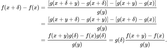
The final expression must go to zero as ${\displaystyle \delta \to 0}$ since ${\displaystyle g(0)=0}$ and ${\displaystyle g(x)}$ is continuous. It follows that ${\displaystyle f(x)}$ is continuous.