Sequence of differential equation solutions
Complex color plot of L − 1/9z 4 ) from − 2− 2i to 2+2i In mathematics , the Laguerre polynomials , named after Edmond Laguerre (1834–1886), are nontrivial solutions of Laguerre's differential equation:
x
y
″
+
(
1
−
x
)
y
′
+
n
y
=
0
,
y
=
L
(
x
)
{\displaystyle xy''+(1-x)y'+ny=0,\ y=L(x)}
linear differential equation . This equation has nonsingular solutions only if n is a non-negative integer.
Sometimes the name Laguerre polynomials is used for solutions of
x
y
″
+
(
α
+
1
−
x
)
y
′
+
n
y
=
0
.
{\displaystyle xy''+(\alpha +1-x)y'+ny=0~.}
n is still a non-negative integer.
Then they are also named generalized Laguerre polynomials , as will be done here (alternatively associated Laguerre polynomials or, rarely, Sonine polynomials , after their inventor Nikolay Yakovlevich Sonin ).
More generally, a Laguerre function is a solution when n is not necessarily a non-negative integer.
The Laguerre polynomials are also used for Gauss–Laguerre quadrature to numerically compute integrals of the form
∫
0
∞
f
(
x
)
e
−
x
d
x
.
{\displaystyle \int _{0}^{\infty }f(x)e^{-x}\,dx.}
These polynomials, usually denoted L 0 L 1 ..., are a polynomial sequence which may be defined by the Rodrigues formula ,
L
n
(
x
)
=
e
x
n
!
d
n
d
x
n
(
e
−
x
x
n
)
=
1
n
!
(
d
d
x
−
1
)
n
x
n
,
{\displaystyle L_{n}(x)={\frac {e^{x}}{n!}}{\frac {d^{n}}{dx^{n}}}\left(e^{-x}x^{n}\right)={\frac {1}{n!}}\left({\frac {d}{dx}}-1\right)^{n}x^{n},}
They are orthogonal polynomials with respect to an inner product
⟨
f
,
g
⟩
=
∫
0
∞
f
(
x
)
g
(
x
)
e
−
x
d
x
.
{\displaystyle \langle f,g\rangle =\int _{0}^{\infty }f(x)g(x)e^{-x}\,dx.}
The rook polynomials in combinatorics are more or less the same as Laguerre polynomials, up to elementary changes of variables. Further see the Tricomi–Carlitz polynomials .
The Laguerre polynomials arise in quantum mechanics, in the radial part of the solution of the Schrödinger equation for a one-electron atom. They also describe the static Wigner functions of oscillator systems in quantum mechanics in phase space . They further enter in the quantum mechanics of the Morse potential and of the 3D isotropic harmonic oscillator .
Physicists sometimes use a definition for the Laguerre polynomials that is larger by a factor of n ! than the definition used here. (Likewise, some physicists may use somewhat different definitions of the so-called associated Laguerre polynomials.)
One can also define the Laguerre polynomials recursively, defining the first two polynomials as
L
0
(
x
)
=
1
{\displaystyle L_{0}(x)=1}
L
1
(
x
)
=
1
−
x
{\displaystyle L_{1}(x)=1-x}
recurrence relation for any k ≥ 1
L
k
+
1
(
x
)
=
(
2
k
+
1
−
x
)
L
k
(
x
)
−
k
L
k
−
1
(
x
)
k
+
1
.
{\displaystyle L_{k+1}(x)={\frac {(2k+1-x)L_{k}(x)-kL_{k-1}(x)}{k+1}}.}
x
L
n
′
(
x
)
=
n
L
n
(
x
)
−
n
L
n
−
1
(
x
)
.
{\displaystyle xL'_{n}(x)=nL_{n}(x)-nL_{n-1}(x).}
In solution of some boundary value problems, the characteristic values can be useful:
L
k
(
0
)
=
1
,
L
k
′
(
0
)
=
−
k
.
{\displaystyle L_{k}(0)=1,L_{k}'(0)=-k.}
The closed form
L
n
(
x
)
=
∑
k
=
0
n
(
n
k
)
(
−
1
)
k
k
!
x
k
.
{\displaystyle L_{n}(x)=\sum _{k=0}^{n}{\binom {n}{k}}{\frac {(-1)^{k}}{k!}}x^{k}.}
The generating function for them likewise follows,
∑
n
=
0
∞
t
n
L
n
(
x
)
=
1
1
−
t
e
−
t
x
/
(
1
−
t
)
.
{\displaystyle \sum _{n=0}^{\infty }t^{n}L_{n}(x)={\frac {1}{1-t}}e^{-tx/(1-t)}.}
L
n
(
x
)
=
1
n
!
e
x
d
n
d
x
n
(
x
n
e
−
x
)
{\displaystyle L_{n}(x)={\frac {1}{n!}}e^{x}{\frac {d^{n}}{dx^{n}}}(x^{n}e^{-x})}
Polynomials of negative index can be expressed using the ones with positive index:
L
−
n
(
x
)
=
e
x
L
n
−
1
(
−
x
)
.
{\displaystyle L_{-n}(x)=e^{x}L_{n-1}(-x).}
A table of the Laguerre polynomials
n
L
n
(
x
)
{\displaystyle L_{n}(x)\,}
0
1
{\displaystyle 1\,}
1
−
x
+
1
{\displaystyle -x+1\,}
2
1
2
(
x
2
−
4
x
+
2
)
{\displaystyle {\tfrac {1}{2}}(x^{2}-4x+2)\,}
3
1
6
(
−
x
3
+
9
x
2
−
18
x
+
6
)
{\displaystyle {\tfrac {1}{6}}(-x^{3}+9x^{2}-18x+6)\,}
4
1
24
(
x
4
−
16
x
3
+
72
x
2
−
96
x
+
24
)
{\displaystyle {\tfrac {1}{24}}(x^{4}-16x^{3}+72x^{2}-96x+24)\,}
5
1
120
(
−
x
5
+
25
x
4
−
200
x
3
+
600
x
2
−
600
x
+
120
)
{\displaystyle {\tfrac {1}{120}}(-x^{5}+25x^{4}-200x^{3}+600x^{2}-600x+120)\,}
6
1
720
(
x
6
−
36
x
5
+
450
x
4
−
2400
x
3
+
5400
x
2
−
4320
x
+
720
)
{\displaystyle {\tfrac {1}{720}}(x^{6}-36x^{5}+450x^{4}-2400x^{3}+5400x^{2}-4320x+720)\,}
7
1
5040
(
−
x
7
+
49
x
6
−
882
x
5
+
7350
x
4
−
29400
x
3
+
52920
x
2
−
35280
x
+
5040
)
{\displaystyle {\tfrac {1}{5040}}(-x^{7}+49x^{6}-882x^{5}+7350x^{4}-29400x^{3}+52920x^{2}-35280x+5040)\,}
8
1
40320
(
x
8
−
64
x
7
+
1568
x
6
−
18816
x
5
+
117600
x
4
−
376320
x
3
+
564480
x
2
−
322560
x
+
40320
)
{\displaystyle {\tfrac {1}{40320}}(x^{8}-64x^{7}+1568x^{6}-18816x^{5}+117600x^{4}-376320x^{3}+564480x^{2}-322560x+40320)\,}
9
1
362880
(
−
x
9
+
81
x
8
−
2592
x
7
+
42336
x
6
−
381024
x
5
+
1905120
x
4
−
5080320
x
3
+
6531840
x
2
−
3265920
x
+
362880
)
{\displaystyle {\tfrac {1}{362880}}(-x^{9}+81x^{8}-2592x^{7}+42336x^{6}-381024x^{5}+1905120x^{4}-5080320x^{3}+6531840x^{2}-3265920x+362880)\,}
10
1
3628800
(
x
10
−
100
x
9
+
4050
x
8
−
86400
x
7
+
1058400
x
6
−
7620480
x
5
+
31752000
x
4
−
72576000
x
3
+
81648000
x
2
−
36288000
x
+
3628800
)
{\displaystyle {\tfrac {1}{3628800}}(x^{10}-100x^{9}+4050x^{8}-86400x^{7}+1058400x^{6}-7620480x^{5}+31752000x^{4}-72576000x^{3}+81648000x^{2}-36288000x+3628800)\,}
n
1
n
!
(
(
−
x
)
n
+
n
2
(
−
x
)
n
−
1
+
⋯
+
(
n
k
)
2
k
!
(
−
x
)
n
−
k
+
⋯
+
n
(
n
!
)
(
−
x
)
+
n
!
)
{\displaystyle {\tfrac {1}{n!}}((-x)^{n}+n^{2}(-x)^{n-1}+\dots +{\binom {n}{k}}^{2}{k!}(-x)^{n-k}+\dots +n({n!})(-x)+n!)\,}
The first six Laguerre polynomials. Generalized Laguerre polynomials
For arbitrary real α the polynomial solutions of the differential equation
x
y
″
+
(
α
+
1
−
x
)
y
′
+
n
y
=
0
{\displaystyle x\,y''+\left(\alpha +1-x\right)y'+n\,y=0}
generalized Laguerre polynomials , or associated Laguerre polynomials .
One can also define the generalized Laguerre polynomials recursively, defining the first two polynomials as
L
0
(
α
)
(
x
)
=
1
{\displaystyle L_{0}^{(\alpha )}(x)=1}
L
1
(
α
)
(
x
)
=
1
+
α
−
x
{\displaystyle L_{1}^{(\alpha )}(x)=1+\alpha -x}
and then using the following recurrence relation for any k ≥ 1
L
k
+
1
(
α
)
(
x
)
=
(
2
k
+
1
+
α
−
x
)
L
k
(
α
)
(
x
)
−
(
k
+
α
)
L
k
−
1
(
α
)
(
x
)
k
+
1
.
{\displaystyle L_{k+1}^{(\alpha )}(x)={\frac {(2k+1+\alpha -x)L_{k}^{(\alpha )}(x)-(k+\alpha )L_{k-1}^{(\alpha )}(x)}{k+1}}.}
The simple Laguerre polynomials are the special case α = 0
L
n
(
0
)
(
x
)
=
L
n
(
x
)
.
{\displaystyle L_{n}^{(0)}(x)=L_{n}(x).}
The Rodrigues formula for them is
L
n
(
α
)
(
x
)
=
x
−
α
e
x
n
!
d
n
d
x
n
(
e
−
x
x
n
+
α
)
=
x
−
α
n
!
(
d
d
x
−
1
)
n
x
n
+
α
.
{\displaystyle L_{n}^{(\alpha )}(x)={x^{-\alpha }e^{x} \over n!}{d^{n} \over dx^{n}}\left(e^{-x}x^{n+\alpha }\right)={\frac {x^{-\alpha }}{n!}}\left({\frac {d}{dx}}-1\right)^{n}x^{n+\alpha }.}
The generating function for them is
∑
n
=
0
∞
t
n
L
n
(
α
)
(
x
)
=
1
(
1
−
t
)
α
+
1
e
−
t
x
/
(
1
−
t
)
.
{\displaystyle \sum _{n=0}^{\infty }t^{n}L_{n}^{(\alpha )}(x)={\frac {1}{(1-t)^{\alpha +1}}}e^{-tx/(1-t)}.}
The first few generalized Laguerre polynomials, Ln (k ) (x ) Properties
Laguerre functions are defined by confluent hypergeometric functions and Kummer's transformation as
L
n
(
α
)
(
x
)
:=
(
n
+
α
n
)
M
(
−
n
,
α
+
1
,
x
)
.
{\displaystyle L_{n}^{(\alpha )}(x):={n+\alpha \choose n}M(-n,\alpha +1,x).}
(
n
+
α
n
)
{\textstyle {n+\alpha \choose n}}
binomial coefficient . When n is an integer the function reduces to a polynomial of degree n .
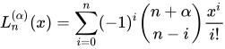
The closed form for these generalized Laguerre polynomials of degree n is
L
n
(
α
)
(
x
)
=
∑
i
=
0
n
(
−
1
)
i
(
n
+
α
n
−
i
)
x
i
i
!
{\displaystyle L_{n}^{(\alpha )}(x)=\sum _{i=0}^{n}(-1)^{i}{n+\alpha \choose n-i}{\frac {x^{i}}{i!}}}
Leibniz's theorem for differentiation of a product to Rodrigues' formula.
Laguerre polynomials have a differential operator representation, much like the closely related Hermite polynomials. Namely, let
D
=
d
d
x
{\displaystyle D={\frac {d}{dx}}}
M
=
x
D
2
+
(
α
+
1
)
D
{\displaystyle M=xD^{2}+(\alpha +1)D}
exp
(
−
t
M
)
x
n
=
(
−
1
)
n
t
n
n
!
L
n
(
α
)
(
x
t
)
{\displaystyle \exp(-tM)x^{n}=(-1)^{n}t^{n}n!L_{n}^{(\alpha )}\left({\frac {x}{t}}\right)}
[ citation needed ]
The first few generalized Laguerre polynomials are:
n
L
n
(
α
)
(
x
)
{\displaystyle L_{n}^{(\alpha )}(x)\,}
0
1
{\displaystyle 1\,}
1
−
x
+
α
+
1
{\displaystyle -x+\alpha +1\,}
2
1
2
(
x
2
−
2
(
α
+
2
)
x
+
(
α
+
1
)
(
α
+
2
)
)
{\displaystyle {\tfrac {1}{2}}(x^{2}-2\left(\alpha +2\right)x+\left(\alpha +1\right)\left(\alpha +2\right))\,}
3
1
6
(
−
x
3
+
3
(
α
+
3
)
x
2
−
3
(
α
+
2
)
(
α
+
3
)
x
+
(
α
+
1
)
(
α
+
2
)
(
α
+
3
)
)
{\displaystyle {\tfrac {1}{6}}(-x^{3}+3\left(\alpha +3\right)x^{2}-3\left(\alpha +2\right)\left(\alpha +3\right)x+\left(\alpha +1\right)\left(\alpha +2\right)\left(\alpha +3\right))\,}
4
1
24
(
x
4
−
4
(
α
+
4
)
x
3
+
6
(
α
+
3
)
(
α
+
4
)
x
2
−
4
(
α
+
2
)
⋯
(
α
+
4
)
x
+
(
α
+
1
)
⋯
(
α
+
4
)
)
{\displaystyle {\tfrac {1}{24}}(x^{4}-4\left(\alpha +4\right)x^{3}+6\left(\alpha +3\right)\left(\alpha +4\right)x^{2}-4\left(\alpha +2\right)\cdots \left(\alpha +4\right)x+\left(\alpha +1\right)\cdots \left(\alpha +4\right))\,}
5
1
120
(
−
x
5
+
5
(
α
+
5
)
x
4
−
10
(
α
+
4
)
(
α
+
5
)
x
3
+
10
(
α
+
3
)
⋯
(
α
+
5
)
x
2
−
5
(
α
+
2
)
⋯
(
α
+
5
)
x
+
(
α
+
1
)
⋯
(
α
+
5
)
)
{\displaystyle {\tfrac {1}{120}}(-x^{5}+5\left(\alpha +5\right)x^{4}-10\left(\alpha +4\right)\left(\alpha +5\right)x^{3}+10\left(\alpha +3\right)\cdots \left(\alpha +5\right)x^{2}-5\left(\alpha +2\right)\cdots \left(\alpha +5\right)x+\left(\alpha +1\right)\cdots \left(\alpha +5\right))\,}
6
1
720
(
x
6
−
6
(
α
+
6
)
x
5
+
15
(
α
+
5
)
(
α
+
6
)
x
4
−
20
(
α
+
4
)
⋯
(
α
+
6
)
x
3
+
15
(
α
+
3
)
⋯
(
α
+
6
)
x
2
−
6
(
α
+
2
)
⋯
(
α
+
6
)
x
+
(
α
+
1
)
⋯
(
α
+
6
)
)
{\displaystyle {\tfrac {1}{720}}(x^{6}-6\left(\alpha +6\right)x^{5}+15\left(\alpha +5\right)\left(\alpha +6\right)x^{4}-20\left(\alpha +4\right)\cdots \left(\alpha +6\right)x^{3}+15\left(\alpha +3\right)\cdots \left(\alpha +6\right)x^{2}-6\left(\alpha +2\right)\cdots \left(\alpha +6\right)x+\left(\alpha +1\right)\cdots \left(\alpha +6\right))\,}
7
1
5040
(
−
x
7
+
7
(
α
+
7
)
x
6
−
21
(
α
+
6
)
(
α
+
7
)
x
5
+
35
(
α
+
5
)
⋯
(
α
+
7
)
x
4
−
35
(
α
+
4
)
⋯
(
α
+
7
)
x
3
+
21
(
α
+
3
)
⋯
(
α
+
7
)
x
2
−
7
(
α
+
2
)
⋯
(
α
+
7
)
x
+
(
α
+
1
)
⋯
(
α
+
7
)
)
{\displaystyle {\tfrac {1}{5040}}(-x^{7}+7\left(\alpha +7\right)x^{6}-21\left(\alpha +6\right)\left(\alpha +7\right)x^{5}+35\left(\alpha +5\right)\cdots \left(\alpha +7\right)x^{4}-35\left(\alpha +4\right)\cdots \left(\alpha +7\right)x^{3}+21\left(\alpha +3\right)\cdots \left(\alpha +7\right)x^{2}-7\left(\alpha +2\right)\cdots \left(\alpha +7\right)x+\left(\alpha +1\right)\cdots \left(\alpha +7\right))\,}
8
1
40320
(
x
8
−
8
(
α
+
8
)
x
7
+
28
(
α
+
7
)
(
α
+
8
)
x
6
−
56
(
α
+
6
)
⋯
(
α
+
8
)
x
5
+
70
(
α
+
5
)
⋯
(
α
+
8
)
x
4
−
56
(
α
+
4
)
⋯
(
α
+
8
)
x
3
+
28
(
α
+
3
)
⋯
(
α
+
8
)
x
2
−
8
(
α
+
2
)
⋯
(
α
+
8
)
x
+
(
α
+
1
)
⋯
(
α
+
8
)
)
{\displaystyle {\tfrac {1}{40320}}(x^{8}-8\left(\alpha +8\right)x^{7}+28\left(\alpha +7\right)\left(\alpha +8\right)x^{6}-56\left(\alpha +6\right)\cdots \left(\alpha +8\right)x^{5}+70\left(\alpha +5\right)\cdots \left(\alpha +8\right)x^{4}-56\left(\alpha +4\right)\cdots \left(\alpha +8\right)x^{3}+28\left(\alpha +3\right)\cdots \left(\alpha +8\right)x^{2}-8\left(\alpha +2\right)\cdots \left(\alpha +8\right)x+\left(\alpha +1\right)\cdots \left(\alpha +8\right))\,}
9
1
362880
(
−
x
9
+
9
(
α
+
9
)
x
8
−
36
(
α
+
8
)
(
α
+
9
)
x
7
+
84
(
α
+
7
)
⋯
(
α
+
9
)
x
6
−
126
(
α
+
6
)
⋯
(
α
+
9
)
x
5
+
126
(
α
+
5
)
⋯
(
α
+
9
)
x
4
−
84
(
α
+
4
)
⋯
(
α
+
9
)
x
3
+
36
(
α
+
3
)
⋯
(
α
+
9
)
x
2
−
9
(
α
+
2
)
⋯
(
α
+
9
)
x
+
(
α
+
1
)
⋯
(
α
+
9
)
)
{\displaystyle {\tfrac {1}{362880}}(-x^{9}+9\left(\alpha +9\right)x^{8}-36\left(\alpha +8\right)\left(\alpha +9\right)x^{7}+84\left(\alpha +7\right)\cdots \left(\alpha +9\right)x^{6}-126\left(\alpha +6\right)\cdots \left(\alpha +9\right)x^{5}+126\left(\alpha +5\right)\cdots \left(\alpha +9\right)x^{4}-84\left(\alpha +4\right)\cdots \left(\alpha +9\right)x^{3}+36\left(\alpha +3\right)\cdots \left(\alpha +9\right)x^{2}-9\left(\alpha +2\right)\cdots \left(\alpha +9\right)x+\left(\alpha +1\right)\cdots \left(\alpha +9\right))\,}
10
1
3628800
(
x
10
−
10
(
α
+
10
)
x
9
+
45
(
α
+
9
)
(
α
+
10
)
x
8
−
120
(
α
+
8
)
⋯
(
α
+
10
)
x
7
+
210
(
α
+
7
)
⋯
(
α
+
10
)
x
6
−
252
(
α
+
6
)
⋯
(
α
+
10
)
x
5
+
210
(
α
+
5
)
⋯
(
α
+
10
)
x
4
−
120
(
α
+
4
)
⋯
(
α
+
10
)
x
3
+
45
(
α
+
3
)
⋯
(
α
+
10
)
x
2
−
10
(
α
+
2
)
⋯
(
α
+
10
)
x
+
(
α
+
1
)
⋯
(
α
+
10
)
)
{\displaystyle {\tfrac {1}{3628800}}(x^{10}-10\left(\alpha +10\right)x^{9}+45\left(\alpha +9\right)\left(\alpha +10\right)x^{8}-120\left(\alpha +8\right)\cdots \left(\alpha +10\right)x^{7}+210\left(\alpha +7\right)\cdots \left(\alpha +10\right)x^{6}-252\left(\alpha +6\right)\cdots \left(\alpha +10\right)x^{5}+210\left(\alpha +5\right)\cdots \left(\alpha +10\right)x^{4}-120\left(\alpha +4\right)\cdots \left(\alpha +10\right)x^{3}+45\left(\alpha +3\right)\cdots \left(\alpha +10\right)x^{2}-10\left(\alpha +2\right)\cdots \left(\alpha +10\right)x+\left(\alpha +1\right)\cdots \left(\alpha +10\right))\,}
The coefficient of the leading term is (−1)n n ! ;
The constant term , which is the value at 0, is
L
n
(
α
)
(
0
)
=
(
n
+
α
n
)
=
Γ
(
n
+
α
+
1
)
n
!
Γ
(
α
+
1
)
;
{\displaystyle L_{n}^{(\alpha )}(0)={n+\alpha \choose n}={\frac {\Gamma (n+\alpha +1)}{n!\,\Gamma (\alpha +1)}};}
The discriminant is
Disc
(
L
n
(
α
)
)
=
∏
j
=
1
n
j
j
−
2
n
+
2
(
j
+
α
)
j
−
1
{\displaystyle \operatorname {Disc} \left(L_{n}^{(\alpha )}\right)=\prod _{j=1}^{n}j^{j-2n+2}(j+\alpha )^{j-1}}
As a contour integral
Given the generating function specified above, the polynomials may be expressed in terms of a contour integral
L
n
(
α
)
(
x
)
=
1
2
π
i
∮
C
e
−
x
t
/
(
1
−
t
)
(
1
−
t
)
α
+
1
t
n
+
1
d
t
,
{\displaystyle L_{n}^{(\alpha )}(x)={\frac {1}{2\pi i}}\oint _{C}{\frac {e^{-xt/(1-t)}}{(1-t)^{\alpha +1}\,t^{n+1}}}\;dt,}
essential singularity at 1
Recurrence relations
The addition formula for Laguerre polynomials:
L
n
(
α
1
+
⋯
+
α
r
+
r
−
1
)
(
x
1
+
⋯
+
x
r
)
=
∑
m
1
+
⋯
+
m
r
=
n
L
m
1
(
α
1
)
(
x
1
)
⋯
L
m
r
(
α
r
)
(
x
r
)
.
{\displaystyle L_{n}^{(\alpha _{1}+\dots +\alpha _{r}+r-1)}\left(x_{1}+\dots +x_{r}\right)=\sum _{m_{1}+\dots +m_{r}=n}L_{m_{1}}^{(\alpha _{1})}\left(x_{1}\right)\cdots L_{m_{r}}^{(\alpha _{r})}\left(x_{r}\right).}
L
n
(
α
)
(
x
)
=
∑
i
=
0
n
L
n
−
i
(
α
+
i
)
(
y
)
(
y
−
x
)
i
i
!
,
{\displaystyle L_{n}^{(\alpha )}(x)=\sum _{i=0}^{n}L_{n-i}^{(\alpha +i)}(y){\frac {(y-x)^{i}}{i!}},}
L
n
(
α
+
1
)
(
x
)
=
∑
i
=
0
n
L
i
(
α
)
(
x
)
{\displaystyle L_{n}^{(\alpha +1)}(x)=\sum _{i=0}^{n}L_{i}^{(\alpha )}(x)}
L
n
(
α
)
(
x
)
=
∑
i
=
0
n
(
α
−
β
+
n
−
i
−
1
n
−
i
)
L
i
(
β
)
(
x
)
,
{\displaystyle L_{n}^{(\alpha )}(x)=\sum _{i=0}^{n}{\alpha -\beta +n-i-1 \choose n-i}L_{i}^{(\beta )}(x),}
L
n
(
α
)
(
x
)
=
∑
i
=
0
n
(
α
−
β
+
n
n
−
i
)
L
i
(
β
−
i
)
(
x
)
;
{\displaystyle L_{n}^{(\alpha )}(x)=\sum _{i=0}^{n}{\alpha -\beta +n \choose n-i}L_{i}^{(\beta -i)}(x);}
L
n
(
α
)
(
x
)
−
∑
j
=
0
Δ
−
1
(
n
+
α
n
−
j
)
(
−
1
)
j
x
j
j
!
=
(
−
1
)
Δ
x
Δ
(
Δ
−
1
)
!
∑
i
=
0
n
−
Δ
(
n
+
α
n
−
Δ
−
i
)
(
n
−
i
)
(
n
i
)
L
i
(
α
+
Δ
)
(
x
)
=
(
−
1
)
Δ
x
Δ
(
Δ
−
1
)
!
∑
i
=
0
n
−
Δ
(
n
+
α
−
i
−
1
n
−
Δ
−
i
)
(
n
−
i
)
(
n
i
)
L
i
(
n
+
α
+
Δ
−
i
)
(
x
)
{\displaystyle {\begin{aligned}L_{n}^{(\alpha )}(x)-\sum _{j=0}^{\Delta -1}{n+\alpha \choose n-j}(-1)^{j}{\frac {x^{j}}{j!}}&=(-1)^{\Delta }{\frac {x^{\Delta }}{(\Delta -1)!}}\sum _{i=0}^{n-\Delta }{\frac {n+\alpha \choose n-\Delta -i}{(n-i){n \choose i}}}L_{i}^{(\alpha +\Delta )}(x)\\[6pt]&=(-1)^{\Delta }{\frac {x^{\Delta }}{(\Delta -1)!}}\sum _{i=0}^{n-\Delta }{\frac {n+\alpha -i-1 \choose n-\Delta -i}{(n-i){n \choose i}}}L_{i}^{(n+\alpha +\Delta -i)}(x)\end{aligned}}}
They can be used to derive the four 3-point-rules
L
n
(
α
)
(
x
)
=
L
n
(
α
+
1
)
(
x
)
−
L
n
−
1
(
α
+
1
)
(
x
)
=
∑
j
=
0
k
(
k
j
)
(
−
1
)
j
L
n
−
j
(
α
+
k
)
(
x
)
,
n
L
n
(
α
)
(
x
)
=
(
n
+
α
)
L
n
−
1
(
α
)
(
x
)
−
x
L
n
−
1
(
α
+
1
)
(
x
)
,
or
x
k
k
!
L
n
(
α
)
(
x
)
=
∑
i
=
0
k
(
−
1
)
i
(
n
+
i
i
)
(
n
+
α
k
−
i
)
L
n
+
i
(
α
−
k
)
(
x
)
,
n
L
n
(
α
+
1
)
(
x
)
=
(
n
−
x
)
L
n
−
1
(
α
+
1
)
(
x
)
+
(
n
+
α
)
L
n
−
1
(
α
)
(
x
)
x
L
n
(
α
+
1
)
(
x
)
=
(
n
+
α
)
L
n
−
1
(
α
)
(
x
)
−
(
n
−
x
)
L
n
(
α
)
(
x
)
;
{\displaystyle {\begin{aligned}L_{n}^{(\alpha )}(x)&=L_{n}^{(\alpha +1)}(x)-L_{n-1}^{(\alpha +1)}(x)=\sum _{j=0}^{k}{k \choose j}(-1)^{j}L_{n-j}^{(\alpha +k)}(x),\\[10pt]nL_{n}^{(\alpha )}(x)&=(n+\alpha )L_{n-1}^{(\alpha )}(x)-xL_{n-1}^{(\alpha +1)}(x),\\[10pt]&{\text{or }}\\{\frac {x^{k}}{k!}}L_{n}^{(\alpha )}(x)&=\sum _{i=0}^{k}(-1)^{i}{n+i \choose i}{n+\alpha \choose k-i}L_{n+i}^{(\alpha -k)}(x),\\[10pt]nL_{n}^{(\alpha +1)}(x)&=(n-x)L_{n-1}^{(\alpha +1)}(x)+(n+\alpha )L_{n-1}^{(\alpha )}(x)\\[10pt]xL_{n}^{(\alpha +1)}(x)&=(n+\alpha )L_{n-1}^{(\alpha )}(x)-(n-x)L_{n}^{(\alpha )}(x);\end{aligned}}}
combined they give this additional, useful recurrence relations
L
n
(
α
)
(
x
)
=
(
2
+
α
−
1
−
x
n
)
L
n
−
1
(
α
)
(
x
)
−
(
1
+
α
−
1
n
)
L
n
−
2
(
α
)
(
x
)
=
α
+
1
−
x
n
L
n
−
1
(
α
+
1
)
(
x
)
−
x
n
L
n
−
2
(
α
+
2
)
(
x
)
{\displaystyle {\begin{aligned}L_{n}^{(\alpha )}(x)&=\left(2+{\frac {\alpha -1-x}{n}}\right)L_{n-1}^{(\alpha )}(x)-\left(1+{\frac {\alpha -1}{n}}\right)L_{n-2}^{(\alpha )}(x)\\[10pt]&={\frac {\alpha +1-x}{n}}L_{n-1}^{(\alpha +1)}(x)-{\frac {x}{n}}L_{n-2}^{(\alpha +2)}(x)\end{aligned}}}
Since
L
n
(
α
)
(
x
)
{\displaystyle L_{n}^{(\alpha )}(x)}
monic polynomial of degree
n
{\displaystyle n}
α
{\displaystyle \alpha }
partial fraction decomposition
n
!
L
n
(
α
)
(
x
)
(
α
+
1
)
n
=
1
−
∑
j
=
1
n
(
−
1
)
j
j
α
+
j
(
n
j
)
L
n
(
−
j
)
(
x
)
=
1
−
∑
j
=
1
n
x
j
α
+
j
L
n
−
j
(
j
)
(
x
)
(
j
−
1
)
!
=
1
−
x
∑
i
=
1
n
L
n
−
i
(
−
α
)
(
x
)
L
i
−
1
(
α
+
1
)
(
−
x
)
α
+
i
.
{\displaystyle {\begin{aligned}{\frac {n!\,L_{n}^{(\alpha )}(x)}{(\alpha +1)_{n}}}&=1-\sum _{j=1}^{n}(-1)^{j}{\frac {j}{\alpha +j}}{n \choose j}L_{n}^{(-j)}(x)\\&=1-\sum _{j=1}^{n}{\frac {x^{j}}{\alpha +j}}\,\,{\frac {L_{n-j}^{(j)}(x)}{(j-1)!}}\\&=1-x\sum _{i=1}^{n}{\frac {L_{n-i}^{(-\alpha )}(x)L_{i-1}^{(\alpha +1)}(-x)}{\alpha +i}}.\end{aligned}}}
i and n and immediate from the expression of
L
n
(
α
)
(
x
)
{\displaystyle L_{n}^{(\alpha )}(x)}
Charlier polynomials :
(
−
x
)
i
i
!
L
n
(
i
−
n
)
(
x
)
=
(
−
x
)
n
n
!
L
i
(
n
−
i
)
(
x
)
.
{\displaystyle {\frac {(-x)^{i}}{i!}}L_{n}^{(i-n)}(x)={\frac {(-x)^{n}}{n!}}L_{i}^{(n-i)}(x).}
Derivatives
Differentiating the power series representation of a generalized Laguerre polynomial k times leads to
d
k
d
x
k
L
n
(
α
)
(
x
)
=
{
(
−
1
)
k
L
n
−
k
(
α
+
k
)
(
x
)
if
k
≤
n
,
0
otherwise.
{\displaystyle {\frac {d^{k}}{dx^{k}}}L_{n}^{(\alpha )}(x)={\begin{cases}(-1)^{k}L_{n-k}^{(\alpha +k)}(x)&{\text{if }}k\leq n,\\0&{\text{otherwise.}}\end{cases}}}
This points to a special case (α = 0α = k
L
n
(
k
)
(
x
)
=
(
−
1
)
k
d
k
L
n
+
k
(
x
)
d
x
k
,
{\displaystyle L_{n}^{(k)}(x)=(-1)^{k}{\frac {d^{k}L_{n+k}(x)}{dx^{k}}},}
k sometimes causing confusion with the usual parenthesis notation for a derivative.
Moreover, the following equation holds:
1
k
!
d
k
d
x
k
x
α
L
n
(
α
)
(
x
)
=
(
n
+
α
k
)
x
α
−
k
L
n
(
α
−
k
)
(
x
)
,
{\displaystyle {\frac {1}{k!}}{\frac {d^{k}}{dx^{k}}}x^{\alpha }L_{n}^{(\alpha )}(x)={n+\alpha \choose k}x^{\alpha -k}L_{n}^{(\alpha -k)}(x),}
Cauchy's formula to
L
n
(
α
′
)
(
x
)
=
(
α
′
−
α
)
(
α
′
+
n
α
′
−
α
)
∫
0
x
t
α
(
x
−
t
)
α
′
−
α
−
1
x
α
′
L
n
(
α
)
(
t
)
d
t
.
{\displaystyle L_{n}^{(\alpha ')}(x)=(\alpha '-\alpha ){\alpha '+n \choose \alpha '-\alpha }\int _{0}^{x}{\frac {t^{\alpha }(x-t)^{\alpha '-\alpha -1}}{x^{\alpha '}}}L_{n}^{(\alpha )}(t)\,dt.}
The derivative with respect to the second variable α has the form,
d
d
α
L
n
(
α
)
(
x
)
=
∑
i
=
0
n
−
1
L
i
(
α
)
(
x
)
n
−
i
.
{\displaystyle {\frac {d}{d\alpha }}L_{n}^{(\alpha )}(x)=\sum _{i=0}^{n-1}{\frac {L_{i}^{(\alpha )}(x)}{n-i}}.}
x
L
n
(
α
)
′
′
(
x
)
+
(
α
+
1
−
x
)
L
n
(
α
)
′
(
x
)
+
n
L
n
(
α
)
(
x
)
=
0
,
{\displaystyle xL_{n}^{(\alpha )\prime \prime }(x)+(\alpha +1-x)L_{n}^{(\alpha )\prime }(x)+nL_{n}^{(\alpha )}(x)=0,}
k th derivative of the ordinary Laguerre polynomial,
x
L
n
[
k
]
′
′
(
x
)
+
(
k
+
1
−
x
)
L
n
[
k
]
′
(
x
)
+
(
n
−
k
)
L
n
[
k
]
(
x
)
=
0
,
{\displaystyle xL_{n}^{[k]\prime \prime }(x)+(k+1-x)L_{n}^{[k]\prime }(x)+(n-k)L_{n}^{[k]}(x)=0,}
L
n
[
k
]
(
x
)
≡
d
k
L
n
(
x
)
d
x
k
{\displaystyle L_{n}^{[k]}(x)\equiv {\frac {d^{k}L_{n}(x)}{dx^{k}}}}
In Sturm–Liouville form the differential equation is
−
(
x
α
+
1
e
−
x
⋅
L
n
(
α
)
(
x
)
′
)
′
=
n
⋅
x
α
e
−
x
⋅
L
n
(
α
)
(
x
)
,
{\displaystyle -\left(x^{\alpha +1}e^{-x}\cdot L_{n}^{(\alpha )}(x)^{\prime }\right)'=n\cdot x^{\alpha }e^{-x}\cdot L_{n}^{(\alpha )}(x),}
which shows that L (α) n n .
Orthogonality
The generalized Laguerre polynomials are orthogonal over [ 0, ∞)weighting function xα e −x
∫
0
∞
x
α
e
−
x
L
n
(
α
)
(
x
)
L
m
(
α
)
(
x
)
d
x
=
Γ
(
n
+
α
+
1
)
n
!
δ
n
,
m
,
{\displaystyle \int _{0}^{\infty }x^{\alpha }e^{-x}L_{n}^{(\alpha )}(x)L_{m}^{(\alpha )}(x)dx={\frac {\Gamma (n+\alpha +1)}{n!}}\delta _{n,m},}
which follows from
∫
0
∞
x
α
′
−
1
e
−
x
L
n
(
α
)
(
x
)
d
x
=
(
α
−
α
′
+
n
n
)
Γ
(
α
′
)
.
{\displaystyle \int _{0}^{\infty }x^{\alpha '-1}e^{-x}L_{n}^{(\alpha )}(x)dx={\alpha -\alpha '+n \choose n}\Gamma (\alpha ').}
If
Γ
(
x
,
α
+
1
,
1
)
{\displaystyle \Gamma (x,\alpha +1,1)}
gamma distribution then the orthogonality relation can be written as
∫
0
∞
L
n
(
α
)
(
x
)
L
m
(
α
)
(
x
)
Γ
(
x
,
α
+
1
,
1
)
d
x
=
(
n
+
α
n
)
δ
n
,
m
.
{\displaystyle \int _{0}^{\infty }L_{n}^{(\alpha )}(x)L_{m}^{(\alpha )}(x)\Gamma (x,\alpha +1,1)dx={n+\alpha \choose n}\delta _{n,m}.}
The associated, symmetric kernel polynomial has the representations (Christoffel–Darboux formula )[ citation needed ]
K
n
(
α
)
(
x
,
y
)
:=
1
Γ
(
α
+
1
)
∑
i
=
0
n
L
i
(
α
)
(
x
)
L
i
(
α
)
(
y
)
(
α
+
i
i
)
=
1
Γ
(
α
+
1
)
L
n
(
α
)
(
x
)
L
n
+
1
(
α
)
(
y
)
−
L
n
+
1
(
α
)
(
x
)
L
n
(
α
)
(
y
)
x
−
y
n
+
1
(
n
+
α
n
)
=
1
Γ
(
α
+
1
)
∑
i
=
0
n
x
i
i
!
L
n
−
i
(
α
+
i
)
(
x
)
L
n
−
i
(
α
+
i
+
1
)
(
y
)
(
α
+
n
n
)
(
n
i
)
;
{\displaystyle {\begin{aligned}K_{n}^{(\alpha )}(x,y)&:={\frac {1}{\Gamma (\alpha +1)}}\sum _{i=0}^{n}{\frac {L_{i}^{(\alpha )}(x)L_{i}^{(\alpha )}(y)}{\alpha +i \choose i}}\\[4pt]&={\frac {1}{\Gamma (\alpha +1)}}{\frac {L_{n}^{(\alpha )}(x)L_{n+1}^{(\alpha )}(y)-L_{n+1}^{(\alpha )}(x)L_{n}^{(\alpha )}(y)}{{\frac {x-y}{n+1}}{n+\alpha \choose n}}}\\[4pt]&={\frac {1}{\Gamma (\alpha +1)}}\sum _{i=0}^{n}{\frac {x^{i}}{i!}}{\frac {L_{n-i}^{(\alpha +i)}(x)L_{n-i}^{(\alpha +i+1)}(y)}{{\alpha +n \choose n}{n \choose i}}};\end{aligned}}}
recursively
K
n
(
α
)
(
x
,
y
)
=
y
α
+
1
K
n
−
1
(
α
+
1
)
(
x
,
y
)
+
1
Γ
(
α
+
1
)
L
n
(
α
+
1
)
(
x
)
L
n
(
α
)
(
y
)
(
α
+
n
n
)
.
{\displaystyle K_{n}^{(\alpha )}(x,y)={\frac {y}{\alpha +1}}K_{n-1}^{(\alpha +1)}(x,y)+{\frac {1}{\Gamma (\alpha +1)}}{\frac {L_{n}^{(\alpha +1)}(x)L_{n}^{(\alpha )}(y)}{\alpha +n \choose n}}.}
Moreover, by the orthogonality and completeness relation for the generalized Laguerre polynomials, the kernel converges in the sense of distributions:
y
α
e
−
y
K
n
(
α
)
(
⋅
,
y
)
→
δ
(
y
−
⋅
)
,
n
→
∞
.
{\displaystyle y^{\alpha }e^{-y}K_{n}^{(\alpha )}(\cdot ,y)\to \delta (y-\cdot ),\qquad n\to \infty .}
Turán's inequalities can be derived here, which is
L
n
(
α
)
(
x
)
2
−
L
n
−
1
(
α
)
(
x
)
L
n
+
1
(
α
)
(
x
)
=
∑
k
=
0
n
−
1
(
α
+
n
−
1
n
−
k
)
n
(
n
k
)
L
k
(
α
−
1
)
(
x
)
2
>
0.
{\displaystyle L_{n}^{(\alpha )}(x)^{2}-L_{n-1}^{(\alpha )}(x)L_{n+1}^{(\alpha )}(x)=\sum _{k=0}^{n-1}{\frac {\alpha +n-1 \choose n-k}{n{n \choose k}}}L_{k}^{(\alpha -1)}(x)^{2}>0.}
The following integral is needed in the quantum mechanical treatment of the hydrogen atom ,
∫
0
∞
x
α
+
1
e
−
x
[
L
n
(
α
)
(
x
)
]
2
d
x
=
(
n
+
α
)
!
n
!
(
2
n
+
α
+
1
)
.
{\displaystyle \int _{0}^{\infty }x^{\alpha +1}e^{-x}\left[L_{n}^{(\alpha )}(x)\right]^{2}dx={\frac {(n+\alpha )!}{n!}}(2n+\alpha +1).}
Series expansions
Let a function have the (formal) series expansion
f
(
x
)
=
∑
i
=
0
∞
f
i
(
α
)
L
i
(
α
)
(
x
)
.
{\displaystyle f(x)=\sum _{i=0}^{\infty }f_{i}^{(\alpha )}L_{i}^{(\alpha )}(x).}
Then
f
i
(
α
)
=
∫
0
∞
L
i
(
α
)
(
x
)
(
i
+
α
i
)
⋅
x
α
e
−
x
Γ
(
α
+
1
)
⋅
f
(
x
)
d
x
.
{\displaystyle f_{i}^{(\alpha )}=\int _{0}^{\infty }{\frac {L_{i}^{(\alpha )}(x)}{i+\alpha \choose i}}\cdot {\frac {x^{\alpha }e^{-x}}{\Gamma (\alpha +1)}}\cdot f(x)\,dx.}
The series converges in the associated Hilbert space L 2 [0, ∞)if and only if
‖
f
‖
L
2
2
:=
∫
0
∞
x
α
e
−
x
Γ
(
α
+
1
)
|
f
(
x
)
|
2
d
x
=
∑
i
=
0
∞
(
i
+
α
i
)
|
f
i
(
α
)
|
2
<
∞
.
{\displaystyle \|f\|_{L^{2}}^{2}:=\int _{0}^{\infty }{\frac {x^{\alpha }e^{-x}}{\Gamma (\alpha +1)}}|f(x)|^{2}\,dx=\sum _{i=0}^{\infty }{i+\alpha \choose i}|f_{i}^{(\alpha )}|^{2}<\infty .}
Asymptotics
In terms of elementary functions
M
{\displaystyle M}
real number
α
{\displaystyle \alpha }
[
c
,
d
]
⊂
(
0
,
+
∞
)
{\displaystyle [c,d]\subset (0,+\infty )}
x
∈
[
c
,
d
]
{\displaystyle x\in [c,d]}
n
→
∞
{\displaystyle n\to \infty }
L
n
(
α
)
(
x
)
=
n
1
2
α
−
1
4
e
1
2
x
π
1
2
x
1
2
α
+
1
4
(
cos
θ
n
(
α
)
(
x
)
(
∑
m
=
0
M
−
1
a
m
(
x
)
n
1
2
m
+
O
(
1
n
1
2
M
)
)
+
sin
θ
n
(
α
)
(
x
)
(
∑
m
=
1
M
−
1
b
m
(
x
)
n
1
2
m
+
O
(
1
n
1
2
M
)
)
)
{\displaystyle L_{n}^{(\alpha )}\left(x\right)={\frac {n^{{\frac {1}{2}}\alpha -{\frac {1}{4}}}{\mathrm {e} }^{{\frac {1}{2}}x}}{{\pi }^{\frac {1}{2}}x^{{\frac {1}{2}}\alpha +{\frac {1}{4}}}}}\left(\cos \theta _{n}^{(\alpha )}(x)\left(\sum _{m=0}^{M-1}{\frac {a_{m}(x)}{n^{{\frac {1}{2}}m}}}+O\left({\frac {1}{n^{{\frac {1}{2}}M}}}\right)\right)+\sin \theta _{n}^{(\alpha )}(x)\left(\sum _{m=1}^{M-1}{\frac {b_{m}(x)}{n^{{\frac {1}{2}}m}}}+O\left({\frac {1}{n^{{\frac {1}{2}}M}}}\right)\right)\right)}
θ
n
(
α
)
(
x
)
:=
2
(
n
x
)
1
2
−
(
1
2
α
+
1
4
)
π
.
{\displaystyle \theta _{n}^{(\alpha )}(x):=2(nx)^{\frac {1}{2}}-\left({\tfrac {1}{2}}\alpha +{\tfrac {1}{4}}\right)\pi .}
a
0
,
b
1
,
a
1
,
b
2
,
…
{\displaystyle a_{0},b_{1},a_{1},b_{2},\dots }
α
,
x
{\displaystyle \alpha ,x}
n
{\displaystyle n}
x
>
0
{\displaystyle x>0}
a
0
(
x
)
=
1
a
1
(
x
)
=
0
b
1
(
x
)
=
1
48
x
1
2
(
4
x
2
−
24
(
α
+
1
)
x
+
3
−
12
α
2
)
{\displaystyle {\begin{aligned}&a_{0}(x)=1\\&a_{1}(x)=0\\&b_{1}(x)={\frac {1}{48x^{\frac {1}{2}}}}\left(4x^{2}-24(\alpha +1)x+3-12\alpha ^{2}\right)\end{aligned}}}
Perron 's formula.: 78
x
∈
C
∖
[
0
,
∞
)
{\displaystyle x\in \mathbb {C} \setminus [0,\infty )}
Fejér 's formula is a special case of Perron's formula with
M
=
1
{\displaystyle M=1}
In terms of Bessel functions
The Mehler–Heine formula states:
lim
n
→
∞
n
−
α
L
n
(
α
)
(
z
2
4
n
)
=
(
z
2
)
−
α
J
α
(
z
)
,
{\displaystyle \lim _{n\to \infty }n^{-\alpha }L_{n}^{(\alpha )}\left({\frac {z^{2}}{4n}}\right)=\left({\frac {z}{2}}\right)^{-\alpha }J_{\alpha }(z),}
where
J
α
{\displaystyle J_{\alpha }}
Bessel function of the first kind .
See also:.
Zeroes
Inequalities
For
α
>
−
1
{\displaystyle \alpha >-1}
x
1
<
(
α
+
1
)
(
α
+
2
)
n
+
α
+
1
{\displaystyle x_{1}<{\frac {(\alpha +1)(\alpha +2)}{n+\alpha +1}}}
x
1
<
(
α
+
1
)
(
α
+
3
)
2
n
+
α
+
1
{\displaystyle x_{1}<{\frac {(\alpha +1)(\alpha +3)}{2n+\alpha +1}}}
x
1
<
(
α
+
1
)
(
α
+
2
)
(
α
+
4
)
(
2
n
+
α
+
1
)
(
α
+
1
)
2
(
α
+
2
)
+
n
(
5
α
+
11
)
(
n
+
α
+
1
)
{\displaystyle x_{1}<{\frac {(\alpha +1)(\alpha +2)(\alpha +4)(2n+\alpha +1)}{(\alpha +1)^{2}(\alpha +2)+n(5\alpha +11)(n+\alpha +1)}}}
x
n
≤
2
n
+
α
−
1
+
2
(
n
−
2
)
(
n
+
α
−
1
)
{\displaystyle x_{n}\leq 2n+\alpha -1+2{\sqrt {(n-2)(n+\alpha -1)}}}
n
≥
2
{\displaystyle n\geq 2}
x
n
>
4
n
+
α
−
16
2
n
{\displaystyle x_{n}>4n+\alpha -16{\sqrt {2n}}}
x
n
>
3
n
−
4
{\displaystyle x_{n}>3n-4}
x
n
>
2
n
+
α
−
1
{\displaystyle x_{n}>2n+\alpha -1}
x
n
>
2
n
+
α
−
2
+
n
2
−
2
n
+
α
n
+
2
{\displaystyle x_{n}>2n+\alpha -2+{\sqrt {n^{2}-2n+\alpha n+2}}}
(
n
+
2
)
x
1
≥
(
n
−
1
−
n
2
+
(
n
+
2
)
(
α
+
1
)
)
2
−
1
(
n
+
2
)
x
n
≤
(
n
−
1
+
n
2
+
(
n
+
2
)
(
α
+
1
)
)
2
−
1
{\displaystyle {\begin{aligned}&(n+2)x_{1}&\geq \left(n-1-{\sqrt {n^{2}+(n+2)(\alpha +1)}}\right)^{2}-1\\&(n+2)x_{n}&\leq \left(n-1+{\sqrt {n^{2}+(n+2)(\alpha +1)}}\right)^{2}-1\end{aligned}}}
x
1
>
1
2
ν
−
3
−
1
+
4
(
n
−
1
)
(
n
+
α
−
1
)
x
n
<
1
2
ν
−
3
+
1
+
4
(
n
−
1
)
(
n
+
α
−
1
)
{\displaystyle {\begin{aligned}x_{1}&>{\frac {1}{2}}\nu -3-{\sqrt {1+4(n-1)(n+\alpha -1)}}\\x_{n}&<{\frac {1}{2}}\nu -3+{\sqrt {1+4(n-1)(n+\alpha -1)}}\end{aligned}}}
For fixed
k
=
1
,
…
,
n
{\displaystyle k=1,\dots ,n}
ν
x
k
>
j
α
,
k
2
x
k
<
j
α
,
k
2
ν
/
2
+
(
ν
/
2
)
2
−
j
α
,
k
2
if
ν
/
2
>
j
α
,
k
x
k
<
[
ν
1
/
2
+
2
−
1
/
3
ν
−
1
/
6
a
n
−
k
+
1
]
2
if
|
α
|
⩾
1
/
4
x
k
<
ν
+
2
2
3
a
k
ν
1
3
+
2
−
2
3
a
k
2
ν
−
1
3
{\displaystyle {\begin{aligned}\nu x_{k}&>j_{\alpha ,k}^{2}\\x_{k}&<{\frac {j_{\alpha ,k}^{2}}{\nu /2+{\sqrt {(\nu /2)^{2}-j_{\alpha ,k}^{2}}}}}\quad {\text{ if }}\nu /2>j_{\alpha ,k}\\x_{k}&<\left[\nu ^{1/2}+2^{-1/3}\nu ^{-1/6}a_{n-k+1}\right]^{2}\quad {\text{ if }}|\alpha |\geqslant 1/4\\x_{k}&<\nu +2^{\frac {2}{3}}a_{k}\nu ^{\frac {1}{3}}+2^{-{\frac {2}{3}}}a_{k}^{2}\nu ^{-{\frac {1}{3}}}\end{aligned}}}
k
{\displaystyle k}
lim
n
→
∞
ν
x
k
=
j
α
,
k
2
{\displaystyle \lim _{n\to \infty }\nu x_{k}=j_{\alpha ,k}^{2}}
See also.
Electrostatics
The zeroes satisfy the Stieltjes relations
∑
1
≤
j
≤
n
,
i
≠
j
1
x
i
−
x
j
=
1
2
(
1
−
α
+
1
x
i
)
∑
1
≤
j
≤
n
1
x
j
=
n
α
+
1
∑
1
≤
j
≤
n
,
i
≠
j
1
(
x
i
−
x
j
)
2
=
−
(
α
+
1
)
(
α
+
5
)
12
x
i
2
+
2
n
+
α
+
1
6
x
i
−
1
12
∑
1
≤
j
≤
n
,
i
≠
j
1
(
x
i
−
x
j
)
3
=
−
(
α
+
1
)
(
α
+
3
)
8
x
i
3
+
2
n
+
α
+
1
8
x
i
2
{\displaystyle {\begin{aligned}\sum _{1\leq j\leq n,i\neq j}{\frac {1}{x_{i}-x_{j}}}&={\frac {1}{2}}\left(1-{\frac {\alpha +1}{x_{i}}}\right)\\\sum _{1\leq j\leq n}{\frac {1}{x_{j}}}&={\frac {n}{\alpha +1}}\\\sum _{1\leq j\leq n,i\neq j}{\frac {1}{(x_{i}-x_{j})^{2}}}&=-{\frac {(\alpha +1)(\alpha +5)}{12x_{i}^{2}}}+{\frac {2n+\alpha +1}{6x_{i}}}-{\frac {1}{12}}\\\sum _{1\leq j\leq n,i\neq j}{\frac {1}{(x_{i}-x_{j})^{3}}}&=-{\frac {(\alpha +1)(\alpha +3)}{8x_{i}^{3}}}+{\frac {2n+\alpha +1}{8x_{i}^{2}}}\\\end{aligned}}}
+
α
+
1
2
{\displaystyle +{\frac {\alpha +1}{2}}}
electric field of strength
−
1
2
{\displaystyle -{\frac {1}{2}}}
n
{\displaystyle n}
+
1
{\displaystyle +1}
L
n
(
α
)
{\displaystyle L_{n}^{(\alpha )}}
As the zeroes specify the polynomial up to scaling, this provides an alternative way to uniquely characterize the Laguerre polynomials.
The zeroes also satisfy
∑
i
=
1
n
1
x
−
x
i
=
−
∑
k
=
0
∞
S
k
+
1
x
k
,
S
k
:=
∑
i
=
1
n
x
i
−
k
{\displaystyle \sum _{i=1}^{n}{\frac {1}{x-x_{i}}}=-\sum _{k=0}^{\infty }S_{k+1}x^{k},\quad S_{k}:=\sum _{i=1}^{n}x_{i}^{-k}}
S
m
−
1
/
m
<
x
1
<
S
m
/
S
m
+
1
,
m
=
1
,
2
,
…
{\displaystyle S_{m}^{-1/m}<x_{1}<S_{m}/S_{m+1},\quad m=1,2,\ldots }
Limit distribution
Let
F
n
(
t
)
:=
1
n
#
{
i
:
x
i
≤
t
}
{\displaystyle F_{n}(t):={\frac {1}{n}}\#\{i:x_{i}\leq t\}}
cumulative distribution function for the roots, then we have the limit law
lim
n
→
∞
F
n
(
4
n
t
)
=
2
π
∫
0
t
1
−
s
s
d
s
∀
t
∈
(
0
,
1
]
{\displaystyle \lim _{n\to \infty }F_{n}(4nt)={\frac {2}{\pi }}\int _{0}^{t}{\sqrt {\frac {1-s}{s}}}ds\quad \forall t\in (0,1]}
Wishart ensemble spectrum.
For fixed
α
>
−
1
{\displaystyle \alpha >-1}
k
{\displaystyle k}
n
→
∞
{\displaystyle n\to \infty }
x
n
+
1
−
k
=
ν
+
2
2
/
3
a
k
ν
1
/
3
+
1
5
2
4
/
3
a
k
2
ν
−
1
/
3
+
(
11
35
−
α
2
−
12
175
a
k
3
)
ν
−
1
+
(
16
1575
a
k
+
92
7875
a
k
4
)
2
2
/
3
ν
−
5
/
3
−
(
15152
3031875
a
k
5
+
1088
121275
a
k
2
)
2
1
/
3
ν
−
7
/
3
+
O
(
ν
−
3
)
,
{\displaystyle {\begin{aligned}x_{n+1-k}=&\nu +2^{2/3}a_{k}\nu ^{1/3}+{\frac {1}{5}}2^{4/3}a_{k}^{2}\nu ^{-1/3}+\left({\frac {11}{35}}-\alpha ^{2}-{\frac {12}{175}}a_{k}^{3}\right)\nu ^{-1}\\&+\left({\frac {16}{1575}}a_{k}+{\frac {92}{7875}}a_{k}^{4}\right)2^{2/3}\nu ^{-5/3}-\left({\frac {15152}{3031875}}a_{k}^{5}+{\frac {1088}{121275}}a_{k}^{2}\right)2^{1/3}\nu ^{-7/3}+{\mathcal {O}}\left(\nu ^{-3}\right),\end{aligned}}}
For
α
∈
(
−
1
,
0
)
{\displaystyle \alpha \in (-1,0)}
x
1
=
α
+
1
n
+
n
−
1
2
(
α
+
1
n
)
2
−
n
2
+
3
n
−
4
12
(
α
+
1
n
)
3
+
7
n
3
+
6
n
2
+
23
n
−
36
144
(
α
+
1
n
)
4
−
293
n
4
+
210
n
3
+
235
n
2
+
990
n
−
1728
8640
(
α
+
1
n
)
5
+
⋯
{\displaystyle {\begin{aligned}x_{1}={\frac {\alpha +1}{n}}&+{\frac {n-1}{2}}\left({\frac {\alpha +1}{n}}\right)^{2}-{\frac {n^{2}+3n-4}{12}}\left({\frac {\alpha +1}{n}}\right)^{3}\\&+{\frac {7n^{3}+6n^{2}+23n-36}{144}}\left({\frac {\alpha +1}{n}}\right)^{4}\\&-{\frac {293n^{4}+210n^{3}+235n^{2}+990n-1728}{8640}}\left({\frac {\alpha +1}{n}}\right)^{5}+\cdots \end{aligned}}}
Physics convention
The generalized Laguerre polynomials are used to describe the quantum wavefunction for hydrogen atom orbitals. The convention used throughout this article expresses the generalized Laguerre polynomials as
L
n
(
α
)
(
x
)
=
Γ
(
α
+
n
+
1
)
Γ
(
α
+
1
)
n
!
1
F
1
(
−
n
;
α
+
1
;
x
)
,
{\displaystyle L_{n}^{(\alpha )}(x)={\frac {\Gamma (\alpha +n+1)}{\Gamma (\alpha +1)n!}}\,_{1}F_{1}(-n;\alpha +1;x),}
where
1
F
1
(
a
;
b
;
x
)
{\displaystyle \,_{1}F_{1}(a;b;x)}
confluent hypergeometric function .
In the physics literature, the generalized Laguerre polynomials are instead defined as
L
¯
n
(
α
)
(
x
)
=
[
Γ
(
α
+
n
+
1
)
]
2
Γ
(
α
+
1
)
n
!
1
F
1
(
−
n
;
α
+
1
;
x
)
.
{\displaystyle {\bar {L}}_{n}^{(\alpha )}(x)={\frac {\left[\Gamma (\alpha +n+1)\right]^{2}}{\Gamma (\alpha +1)n!}}\,_{1}F_{1}(-n;\alpha +1;x).}
The physics version is related to the standard version by
L
¯
n
(
α
)
(
x
)
=
(
n
+
α
)
!
L
n
(
α
)
(
x
)
.
{\displaystyle {\bar {L}}_{n}^{(\alpha )}(x)=(n+\alpha )!L_{n}^{(\alpha )}(x).}
There is yet another, albeit less frequently used, convention in the physics literature
L
~
n
(
α
)
(
x
)
=
(
−
1
)
α
L
¯
n
−
α
(
α
)
.
{\displaystyle {\tilde {L}}_{n}^{(\alpha )}(x)=(-1)^{\alpha }{\bar {L}}_{n-\alpha }^{(\alpha )}.}



















![{\displaystyle \lim _{n\to \infty }F_{n}(4nt)={\frac {2}{\pi }}\int _{0}^{t}{\sqrt {\frac {1-s}{s}}}ds\quad \forall t\in (0,1]}](https://wikimedia.org/api/rest_v1/media/math/render/svg/dc96768dcdede1c3671f6c52df5b2029ba7407b4)





