Description
Since the vorticity vector  and the velocity vector
 are colinear to each other, we can write

where  is some scalar function. One immediate consequence of Beltrami flow is that it can never be a planar or axisymmetric flow because in those flows, vorticity is always perpendicular to the velocity field. The other important consequence will be realized by looking at the incompressible vorticity equation

where  is an external body forces such as gravitational field, electric field etc., and
 is the kinematic viscosity. Since and are parallel, the non-linear terms in the above equation are equal;
 . Thus Beltrami flows satisfy the linear equations
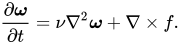
When  , the components of vorticity satisfies a simple heat equation.
Trkalian flow
Viktor Trkal considered the Beltrami flows without any external forces in 1919 for the scalar function  , i.e.,

Introduce the following separation of variables

then the equation satisfied by  becomes

The Chandrasekhar–Kendall functions satisfy this equation.
Berker's solution
Ratip Berker obtained the solution in Cartesian coordinates for in 1963,

Generalized Beltrami flow
The generalized Beltrami flow satisfies the condition

which is less restrictive than the Beltrami condition  . Unlike the normal Beltrami flows, the generalized Beltrami flow can be studied for planar and axisymmetric flows.
Steady planar flows
For steady generalized Beltrami flow, we have  and since it is also planar we have
 . Introduce the stream function

Integration of gives  . So, complete solution is possible if it satisfies all the following three equations

A special case is considered when the flow field has uniform vorticity  . Wang (1991) gave the generalized solution as

assuming a linear function for  . Substituting this into the vorticity equation and introducing the separation of variables
 with the separating constant
 results in

The solution obtained for different choices of  can be interpreted differently, for example,
 represents a flow downstream a uniform grid,
 represents a flow created by a stretching plate,
 represents a flow into a corner,
 represents an Asymptotic suction profile etc.
Unsteady planar flows
Here,
 .
Taylor–Walsh eddies
A family of exact solutions (due to G. I. Taylor (1923) and Owen Walsh (1992); Walsh's solution is of the form  ) is obtained from a separable ansatz in which the whole velocity field decays with a single exponential rate. Let
 be a time-independent field with

For  one has
 , so the unsteady and viscous terms cancel exactly and the momentum equation reduces to
 . Thus is an exact solution if and only if

is a gradient, and then  (up to a function of time): the pressure decays at twice the rate of the velocity. The eigenvalue condition is linear and easy to satisfy; the gradient condition is the real restriction. It holds, for example, for:
- two-dimensional fields whose vorticity is constant along streamlines,
 (Taylor's case below);
- Beltrami flows,
 , for which
 . These include the unsteady Trkal flow and the unsteady versions of the ABC flow and of the Ethier–Steinman flows.
Not every sum of Laplacian eigenmodes works: modes with different eigenvalues decay at different rates, so the shape of the nonlinear term changes in time and in general it cannot be a gradient at all times. These solutions are examples of the generalized Beltrami flows in the sense of Wang. G. I. Taylor originally treated the two-dimensional special case , where  is the vorticity,
 the stream function and
 a constant. The vorticity is then a function of the stream function, so the convective term of the vorticity equation vanishes and the vorticity equation reduces to linear diffusion. He showed that the separation
 satisfies the equation and also
 . As an example he considered a decaying system of eddies rotating alternately in opposite directions in a rectangular array,

where  is the side of the square formed by an eddy, so that

With  ,
 and
 , the pressure is
 .
Steady axisymmetric flows
Here we have  . Integration of gives
 and the three equations are

The first equation is the Hicks equation. Marris and Aswani (1977) showed that the only possible solution is and the remaining equations reduce to

A simple set of solutions to the above equation is

 represents a flow due to two opposing rotational stream on a parabolic surface,
 represents rotational flow on a plane wall,
 represents a flow ellipsoidal vortex (special case – Hill's spherical vortex),
 represents a type of toroidal vortex etc.
The homogeneous solution for  as shown by Berker

where  are the Bessel function of the first kind and Bessel function of the second kind respectively. A special case of the above solution is Poiseuille flow for cylindrical geometry with transpiration velocities on the walls. Chia-Shun Yih found a solution in 1958 for Poiseuille flow into a sink when
 .