Divisor function

In mathematics, and specifically in number theory, a divisor function is an arithmetic function related to the divisors of an integer. When referred to as the divisor function, it counts the number of divisors of an integer (including 1 and the number itself). It appears in a number of remarkable identities, including relationships on the Riemann zeta function and the Eisenstein series of modular forms. Divisor functions were studied by Ramanujan, who gave a number of important congruences and identities; these are treated separately in the article Ramanujan's sum.

A related function is the divisor summatory function, which, as the name implies, is a sum over the divisor function.

Definition

The sum of positive divisors function σ_z(n), for a real or complex number z, is defined as the sum of the zth powers of the positive divisors of n. It can be expressed in sigma notation as

${\displaystyle \sigma _{z}(n)=\sum _{d\mid n}d^{z}\,\!,}$

where ${\displaystyle {d\mid n}}$ is shorthand for "d divides n". The notations d(n), ν(n) and τ(n) (for the German Teiler = divisors) are also used to denote σ₀(n), or the number-of-divisors function (OEIS: A000005). When z is 1, the function is called the sigma function or sum-of-divisors function, and the subscript is often omitted, so σ(n) is the same as σ₁(n) (OEIS: A000203).

The aliquot sum s(n) of n is the sum of the proper divisors (that is, the divisors excluding n itself, OEIS: A001065), and equals σ₁(n) − n; the aliquot sequence of n is formed by repeatedly applying the aliquot sum function.

Example

For example, σ₀(12) is the number of the divisors of 12:

${\displaystyle {\begin{aligned}\sigma _{0}(12)&=1^{0}+2^{0}+3^{0}+4^{0}+6^{0}+12^{0}\\&=1+1+1+1+1+1=6,\end{aligned}}}$

while σ₁(12) is the sum of all the divisors:

${\displaystyle {\begin{aligned}\sigma _{1}(12)&=1^{1}+2^{1}+3^{1}+4^{1}+6^{1}+12^{1}\\&=1+2+3+4+6+12=28,\end{aligned}}}$

and the aliquot sum s(12) of proper divisors is:

${\displaystyle {\begin{aligned}s(12)&=1^{1}+2^{1}+3^{1}+4^{1}+6^{1}\\&=1+2+3+4+6=16.\end{aligned}}}$

σ₋₁(n) is sometimes called the abundancy index of n, and we have:

${\displaystyle {\begin{aligned}\sigma _{-1}(12)&=1^{-1}+2^{-1}+3^{-1}+4^{-1}+6^{-1}+12^{-1}\\[6pt]&={\tfrac {1}{1}}+{\tfrac {1}{2}}+{\tfrac {1}{3}}+{\tfrac {1}{4}}+{\tfrac {1}{6}}+{\tfrac {1}{12}}\\[6pt]&={\tfrac {12}{12}}+{\tfrac {6}{12}}+{\tfrac {4}{12}}+{\tfrac {3}{12}}+{\tfrac {2}{12}}+{\tfrac {1}{12}}\\[6pt]&={\tfrac {12+6+4+3+2+1}{12}}={\tfrac {28}{12}}={\tfrac {7}{3}}={\tfrac {\sigma _{1}(12)}{12}}\end{aligned}}}$

Table of values

The cases x = 2 to 5 are listed in OEIS: A001157 through OEIS: A001160, x = 6 to 24 are listed in OEIS: A013954 through OEIS: A013972.

Properties

Series relations

Two Dirichlet series involving the divisor function are:

${\displaystyle \sum _{n=1}^{\infty }{\frac {\sigma _{a}(n)}{n^{s}}}=\zeta (s)\zeta (s-a)\quad {\text{for}}\quad \Re (s)>1+\max\{\Re (a),0\},}$

where ${\displaystyle \zeta }$ is the Riemann zeta function. The series for d(n) = σ₀(n) gives:

${\displaystyle \sum _{n=1}^{\infty }{\frac {d(n)}{n^{s}}}=\zeta ^{2}(s)\quad {\text{for}}\quad \Re (s)>1,}$

and a Ramanujan identity

${\displaystyle \sum _{n=1}^{\infty }{\frac {\sigma _{a}(n)\sigma _{b}(n)}{n^{s}}}={\frac {\zeta (s)\zeta (s-a)\zeta (s-b)\zeta (s-a-b)}{\zeta (2s-a-b)}},}$

which is a special case of the Rankin–Selberg convolution.

A Lambert series involving the divisor function is:

${\displaystyle \sum _{n=1}^{\infty }q^{n}\sigma _{a}(n)=\sum _{n=1}^{\infty }\sum _{j=1}^{\infty }n^{a}q^{j\,n}=\sum _{n=1}^{\infty }{\frac {n^{a}q^{n}}{1-q^{n}}}=\sum _{n=1}^{\infty }\operatorname {Li} _{-a}(q^{n})}$

for arbitrary complex |q| ≤ 1 and a (${\displaystyle \operatorname {Li} }$ is the polylogarithm). This summation also appears as the Fourier series of the Eisenstein series and the invariants of the Weierstrass elliptic functions.

For ${\displaystyle k>0}$, there is an explicit series representation with Ramanujan sums ${\displaystyle c_{m}(n)}$ as :

${\displaystyle \sigma _{k}(n)=\zeta (k+1)n^{k}\sum _{m=1}^{\infty }{\frac {c_{m}(n)}{m^{k+1}}}.}$

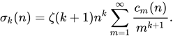
The computation of the first terms of ${\displaystyle c_{m}(n)}$ shows its oscillations around the "average value" ${\displaystyle \zeta (k+1)n^{k}}$:

${\displaystyle \sigma _{k}(n)=\zeta (k+1)n^{k}\left[1+{\frac {(-1)^{n}}{2^{k+1}}}+{\frac {2\cos {\frac {2\pi n}{3}}}{3^{k+1}}}+{\frac {2\cos {\frac {\pi n}{2}}}{4^{k+1}}}+\cdots \right]}$

Growth rate

In little-o notation, the divisor function satisfies the inequality:

${\displaystyle {\mbox{for all }}\varepsilon >0,\quad d(n)=o(n^{\varepsilon }).}$

More precisely, Severin Wigert showed that:

${\displaystyle \limsup _{n\to \infty }{\frac {\log d(n)}{\log n/\log \log n}}=\log 2,}$

approached by ${\displaystyle n}$ taking the primorials since

${\displaystyle p_{k}\#=e^{(1+o(1))k\log k}.}$

On the other hand, since there are infinitely many prime numbers,

${\displaystyle \liminf _{n\to \infty }d(n)=2.}$

In Big-O notation, Peter Gustav Lejeune Dirichlet showed that the average order of the divisor function satisfies the following inequality:

${\displaystyle {\mbox{for all }}x\geq 1,\sum _{n\leq x}d(n)=x\log x+(2\gamma -1)x+O({\sqrt {x}}),}$

where ${\displaystyle \gamma }$ is Euler's gamma constant. Improving the bound ${\displaystyle O({\sqrt {x}})}$ in this formula is known as Dirichlet's divisor problem.

The behaviour of the sigma function is irregular. The asymptotic growth rate of the sigma function can be expressed by:

${\displaystyle \limsup _{n\rightarrow \infty }{\frac {\sigma (n)}{n\,\log \log n}}=e^{\gamma },}$

where lim sup is the limit superior. This result is Grönwall's theorem, published in 1913 (Grönwall 1913). His proof uses Mertens' third theorem, which says that:

${\displaystyle \lim _{n\to \infty }{\frac {1}{\log n}}\prod _{p\leq n}{\frac {p}{p-1}}=e^{\gamma },}$

where p denotes a prime. Grönwall also showed that

${\displaystyle \limsup _{n\rightarrow \infty }{\frac {\sigma _{a}(n)}{n^{a}}}=\zeta (a),\quad a>1,}$

where ${\displaystyle \zeta }$ is the Riemann zeta function.

In 1915, Ramanujan proved that under the assumption of the Riemann hypothesis, Robin's inequality

${\displaystyle \ \sigma (n)<e^{\gamma }n\log \log n}$ (where γ is the Euler–Mascheroni constant)

holds for all sufficiently large n (Ramanujan 1997). The largest known value that violates the inequality is n=5040. In 1984, Guy Robin proved that the inequality is true for all n > 5040 if and only if the Riemann hypothesis is true (Robin 1984). This is Robin's theorem and the inequality became known after him. Robin furthermore showed that if the Riemann hypothesis is false then there are an infinite number of values of n that violate the inequality, and it is known that the smallest such n > 5040 must be superabundant (Akbary & Friggstad 2009). It has been shown that the inequality holds for large odd and square-free integers, and that the Riemann hypothesis is equivalent to the inequality just for n divisible by the fifth power of a prime (Choie et al. 2007).

Robin also proved, unconditionally, that the inequality:

${\displaystyle \ \sigma (n)<e^{\gamma }n\log \log n+{\frac {0.6483\ n}{\log \log n}}}$

holds for all n ≥ 3.

A related bound was given by Jeffrey Lagarias in 2002, who proved that the Riemann hypothesis is equivalent to the statement that:

${\displaystyle \sigma (n)<H_{n}+e^{H_{n}}\log(H_{n})}$

for every natural number n > 1, where ${\displaystyle H_{n}}$ is the nth harmonic number, (Lagarias 2002).

See also

• Divisor sum convolutions, lists a few identities involving the divisor functions
• Euler's totient function, Euler's phi function
• Refactorable number
• Table of divisors
• Unitary divisor

Notes

References

• Akbary, Amir; Friggstad, Zachary (2009), "Superabundant numbers and the Riemann hypothesis" (PDF), American Mathematical Monthly, 116 (3): 273–275, doi:10.4169/193009709X470128, archived from the original (PDF) on 2014-04-11.
• Apostol, Tom M. (1976), Introduction to analytic number theory, Undergraduate Texts in Mathematics, New York-Heidelberg: Springer-Verlag, ISBN 978-0-387-90163-3, MR 0434929, Zbl 0335.10001
• Bach, Eric; Shallit, Jeffrey, Algorithmic Number Theory, volume 1, 1996, MIT Press. ISBN 0-262-02405-5, see page 234 in section 8.8.
• Caveney, Geoffrey; Nicolas, Jean-Louis; Sondow, Jonathan (2011), "Robin's theorem, primes, and a new elementary reformulation of the Riemann Hypothesis" (PDF), INTEGERS: The Electronic Journal of Combinatorial Number Theory, 11: A33, arXiv:1110.5078, Bibcode:2011arXiv1110.5078C
• Choie, YoungJu; Lichiardopol, Nicolas; Moree, Pieter; Solé, Patrick (2007), "On Robin's criterion for the Riemann hypothesis", Journal de théorie des nombres de Bordeaux, 19 (2): 357–372, arXiv:math.NT/0604314, doi:10.5802/jtnb.591, ISSN 1246-7405, MR 2394891, S2CID 3207238, Zbl 1163.11059
• Gioia, A. A.; Vaidya, A. M. (1967), "Amicable numbers with opposite parity", The American Mathematical Monthly, 74 (8): 969–973, doi:10.2307/2315280, JSTOR 2315280, MR 0220659
• Grönwall, Thomas Hakon (1913), "Some asymptotic expressions in the theory of numbers", Transactions of the American Mathematical Society, 14 (1): 113–122, doi:10.1090/S0002-9947-1913-1500940-6
• Hardy, G. H.; Wright, E. M. (2008) [1938], An Introduction to the Theory of Numbers, Revised by D. R. Heath-Brown and J. H. Silverman. Foreword by Andrew Wiles. (6th ed.), Oxford: Oxford University Press, ISBN 978-0-19-921986-5, MR 2445243, Zbl 1159.11001
• Ivić, Aleksandar (1985), The Riemann zeta-function. The theory of the Riemann zeta-function with applications, A Wiley-Interscience Publication, New York etc.: John Wiley & Sons, pp. 385–440, ISBN 0-471-80634-X, Zbl 0556.10026
• Lagarias, Jeffrey C. (2002), "An elementary problem equivalent to the Riemann hypothesis", The American Mathematical Monthly, 109 (6): 534–543, arXiv:math/0008177, doi:10.2307/2695443, ISSN 0002-9890, JSTOR 2695443, MR 1908008, S2CID 15884740
• Long, Calvin T. (1972), Elementary Introduction to Number Theory (2nd ed.), Lexington: D. C. Heath and Company, LCCN 77171950
• Pettofrezzo, Anthony J.; Byrkit, Donald R. (1970), Elements of Number Theory, Englewood Cliffs: Prentice Hall, LCCN 77081766
• Ramanujan, Srinivasa (1997), "Highly composite numbers, annotated by Jean-Louis Nicolas and Guy Robin", The Ramanujan Journal, 1 (2): 119–153, doi:10.1023/A:1009764017495, ISSN 1382-4090, MR 1606180, S2CID 115619659
• Robin, Guy (1984), "Grandes valeurs de la fonction somme des diviseurs et hypothèse de Riemann", Journal de Mathématiques Pures et Appliquées, Neuvième Série, 63 (2): 187–213, ISSN 0021-7824, MR 0774171
• Williams, Kenneth S. (2011), Number theory in the spirit of Liouville, London Mathematical Society Student Texts, vol. 76, Cambridge: Cambridge University Press, ISBN 978-0-521-17562-3, Zbl 1227.11002

External links

• Weisstein, Eric W. "Divisor Function". MathWorld.
• Weisstein, Eric W. "Robin's Theorem". MathWorld.
• Elementary Evaluation of Certain Convolution Sums Involving Divisor Functions PDF of a paper by Huard, Ou, Spearman, and Williams. Contains elementary (i.e. not relying on the theory of modular forms) proofs of divisor sum convolutions, formulas for the number of ways of representing a number as a sum of triangular numbers, and related results.