Kelvin wave

This article may be too technical for most readers to understand. Please help improve it to make it understandable to non-experts, without removing the technical details. (September 2026) (Learn how and when to remove this message)

A Kelvin wave is a low-frequency gravity wave whose motion is concentrated near a vertical boundary (e.g., a shore) or the equator. It occurs in the ocean and the atmosphere, as well as in large lakes. Waves along a coast are called coastal Kelvin waves; those along the equator are equatorial Kelvin waves. In a coastal Kelvin wave, a pressure gradient across the flow balances the Earth's Coriolis force, while the fluid moves along the boundary. Kelvin wave retains its shape as it moves (being, in the shallow water model, non-dispersive), and therefore does not curl over. The direction of the wave is fixed: the coastal wave moves towards the equator along the western coasts, towards the poles along the eastern coasts (like California). Around a closed basin, coastal Kelvin waves travel counterclockwise in the Northern Hemisphere and clockwise in the Southern Hemisphere. Equatorial Kelvin waves always travel eastward.

Kelvin waves are regular events. Both equatorial and coastal waves are observed mutiple times per year. Observations of the equatorial Kelvin wave are important for predictions about El Niño–Southern Oscillation (ENSO), thus the phenomenon attracts attention of the mainstream media. Coastal Kelvin waves are an important component of tide waves.

The Kelvin waves have planetary scale, sometimes thousands of miles long. The equatorial waves move large amounts of heat and are known to temporarily reverse some currents in the upper ocean. At the same time, the height of the equatorial wave (observed changes in the ocean level) is very small: in the Pacific, downwelling Kelvin waves raise sea level by just a few centimetres.

During the meteorological or oceanographical analysis, it can be assumed that one velocity component of a Kelvin wave vanishes (for example, for an equatorial wave there is no flow in the north–south direction), thus making the momentum and continuity equations much simpler). This wave is named after its discoverer, Lord Kelvin (1879).

Surface and internal waves

The Kelvin waves can occur as surface waves (also referred to as barotropic) manifesting themselves as a change in ocean level, and internal (baroclinic) waves, where the interface of a wave is a subsurface change of the water density caused, for example, by a temperature gradient (thermocline).

The surface and internal waves travel in the same direction, but at different speeds:

• the surface waves are fast: in the deep ocean, about 200 m/sec (similar to a tsunami or passenger jet), much slower in the shallow water;
• the internal ocean waves carrying the heat have speed of 1–3 m/sec (similar to a walking or running human). For example, the equatorial internal waves cross the Pacific ocean in about two months. Internal Kelvin waves can produce thermocline displacements with (underwater) amplitudes of approximately 20 metres in the central equatorial Pacific.

The Rossby radius for the coastal barotropic waves is about 3000 kilometers in the deep ocean, 200 kilometers on the continental shelf. The wave height increases as the wave moves into shallower water.

Ubiquity and special events

Kelvin waves occur multiple times per year, but they typically cause very small changes in the sea surface height (SSH) and are "difficult to observe". For example, Kessler et al. note routine occurrence of two to four cases of downwelling equatorial Kelvin waves annually in the Pacific, both in and outside of El Niño. Rao et. al report a cycle of two upwelling and two downwelling equatorial Kelvin waves per year in the Indian ocean that frequently trigger the coastal Kelvin waves.

Flores-Morales et al., after studying 16 years of data, note semiannual pattern of Kelvin wave "signal" originating in the equatorial Pacific and propagating northward along the coast of the tropical Pacific.

Coastal Kelvin waves can temporarily raise sea level. During the 1997–1998 El Niño, Ryan and Noble reported sea-level fluctuations at San Francisco with amplitudes above 10 cm and periods longer than 30 days. They attributed much of this signal to coastally trapped waves originating near the equator, with winds also affecting the observed sea level.

In the 2026 El Niño event, satellite observations detected a series of Kelvin waves crossing the Pacific Ocean. By May, sea surface heights near Peru exceeded their long-term average by more than 15 cm. In October, NOAA reported a coastal Kelvin wave propagating northward along the North American West Coast, with additional waves following across the tropical Pacific.

Relationship with tides

Tidal motion along coastal boundaries can take the form of Kelvin waves. In the idealized description, these waves travel along the coast with their greatest amplitude at the boundary and decreasing amplitude offshore. They propagate with the coast on their right in the Northern Hemisphere and on their left in the Southern Hemisphere.

Incoming Kelvin waves and their reflections explain amphidromic systems, in which the tidal wave appear to move around a central point where its amplitude is zero. In the North Sea, tidal waves enter from the Atlantic, and their propagation and reflection are modified by the shape and depth of the basin and by bottom friction. Models combine Kelvin waves with Poincaré waves in order to reproduce the observed patterns of both diurnal and semidiurnal tides.

Kelvin waves associated with El Niño can also raise coastal sea levels over longer periods, increasing the water levels reached during high tides. During the 1997–1998 El Niño, Kelvin waves raised sea level at San Francisco by approximately 15 cm (5.9 in) as early as May 1997. Elevated sea levels subsequently combined with high tides and storms to worsen coastal flooding.

Equatorial Kelvin wave

Equatorial Kelvin waves travel eastward along the equator and weaken farther north or south (equatorially trapped).

The equator needs no solid boundary to confine these waves. The Coriolis parameter (a measure of Earth's rotational effect on horizontal motion) has opposite signs in the two hemispheres. Eastward flow therefore tends to bring water toward the equator from both sides. Wang describes this as Ekman mass transport (a net sideways movement of water caused by Earth's rotation). Water collecting there creates a meridional pressure gradient (a north–south difference in pressure). Its force opposes the inward Coriolis effect. This balance keeps the wave near the equator, which thus serves a similar purpose to a coast.

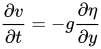
Here, x measures distance eastward along the equator and y measures distance northward from it. The corresponding velocity components are u (east–west flow) and v (north–south flow). The wave extends into both hemispheres. In the ideal Kelvin-wave solution, v is zero, so the wave produces no north–south flow. The primitive equations are identical to those used to develop the coastal Kelvin wave solution (the u- and v-momentum equations and the continuity equation). Because these waves are equatorial, the Coriolis parameter vanishes at 0 degrees; therefore, it is necessary to use the equatorial beta plane approximation:

$${\displaystyle f=\beta y,}$$

where β is the rate at which the Coriolis parameter changes with northward distance at the equator. In this single-layer model, equatorial Kelvin waves travel at ${\displaystyle c={\sqrt {gH}}}$, where H is the mean water depth. For an internal-wave mode, H represents an equivalent depth (an effective depth that gives that mode's wave speed).

For baroclinic waves, a simple reduced-gravity approximation is used, with the ocean represented by two layers, each with uniform density. A lighter upper layer of mean thickness h lies above a much deeper, denser layer, which is assumed to remain at rest. Internal waves displace the interface (the boundary between the layers). For small disturbances, their speed is ${\displaystyle c={\sqrt {g'h}}}$, where g′ is the reduced gravity (gravity multiplied by the fractional density difference between the layers).

The amplitude varies with y as ${\displaystyle \exp(-y^{2}\beta /(2{\sqrt {gH}})).}$ This is a Gaussian profile (a bell-shaped distribution) centered on the equator.

For a depth of four kilometres, the wave speed, ${\displaystyle {\sqrt {gH}},}$ is about 200 metres per second. In the two-layer model this speed is ${\displaystyle c={\sqrt {g'h}}}$; for the first baroclinic mode in the ocean it is typically about 2–3 m/s. At this speed, an equatorial Kelvin wave takes about two months to cross the Pacific Ocean between New Guinea and South America. For higher ocean and atmospheric modes, the phase speeds are comparable to fluid flow speeds.

Both atmospheric^{[citation needed]} and oceanic equatorial Kelvin waves play an important role in the dynamics of El Niño–Southern Oscillation, by transmitting changes in conditions in the Western Pacific to the Eastern Pacific.

There have been studies that connect equatorial Kelvin waves to coastal Kelvin waves. Moore (1968) found that as an equatorial Kelvin wave strikes an "eastern boundary", part of the energy is reflected in the form of planetary and gravity waves; and the remainder of the energy is carried poleward along the eastern boundary as coastal Kelvin waves. This process indicates that some energy may be lost from the equatorial region and transported to the poleward region.

Equatorial Kelvin waves are often associated with anomalies in surface wind stress. For example, positive (eastward) anomalies in wind stress in the central Pacific excite positive anomalies in 20 °C isotherm depth which propagate to the east as equatorial Kelvin waves.

In 2017, Delplace, Marston and Venaille used the shallow water equations to identify a topological origin for equatorial Kelvin waves. Their theoretical analysis related these waves to the one-way boundary states found in topological insulators.

Coastal Kelvin wave

The following derivation describes a surface Kelvin wave using a shallow-water model. The fluid has uniform density and a constant mean depth H, with a vertical wall representing the coast. Its surface displacement from the resting level is η, which varies with position and time. Let a straight coast lie along the y-axis, at x = 0. Take positive x eastward and positive y northward, with the ocean occupying x < 0. The velocity components u and v describe flow perpendicular and parallel to the coast, respectively. Water cannot flow through the coast, so u = 0 there. One may solve a frequency relation for the phase speed of coastal Kelvin waves, which are among the class of waves called boundary waves, edge waves, trapped waves, or surface waves (similar to the Lamb waves). For small surface displacements compared with H, the linearised shallow-water equations are:

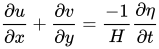
• the continuity equation (accounting for the effects of horizontal convergence and divergence): $${\displaystyle {\frac {\partial u}{\partial x}}+{\frac {\partial v}{\partial y}}={\frac {-1}{H}}{\frac {\partial \eta }{\partial t}}}$$
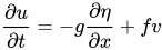
• the u-momentum equation: $${\displaystyle {\frac {\partial u}{\partial t}}=-g{\frac {\partial \eta }{\partial x}}+fv}$$
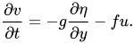
• the v-momentum equation: $${\displaystyle {\frac {\partial v}{\partial t}}=-g{\frac {\partial \eta }{\partial y}}-fu.}$$

in which f is the Coriolis coefficient, which depends on the latitude φ: $${\displaystyle f=2\,\Omega \,\sin \phi }$$ where Ω ≈ 2π / (86164 sec) ≈ 7.292×10⁻⁵ rad/s is the angular speed of rotation of the earth.

For the Kelvin-wave solution, the cross-shore velocity u is assumed to be zero throughout the fluid. The equations then reduce to:

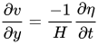
• the continuity equation: $${\displaystyle {\frac {\partial v}{\partial y}}={\frac {-1}{H}}{\frac {\partial \eta }{\partial t}}}$$
• the u-momentum equation: $${\displaystyle g{\frac {\partial \eta }{\partial x}}=fv}$$
• the v-momentum equation: $${\displaystyle {\frac {\partial v}{\partial t}}=-g{\frac {\partial \eta }{\partial y}}}$$

The continuity and alongshore momentum equations allow waves with signed phase velocity ${\displaystyle c=\pm {\sqrt {gH}}}$. The magnitude of c is the speed of shallow-water gravity waves.

For constant f, the Kelvin-wave solution is ${\displaystyle \eta (x,y,t)=W(y-ct)\exp(fx/c)}$, with alongshore velocity ${\displaystyle v=(c/H)\eta }$. Here W sets the wave's profile along the coast. The same signed c appears in the travelling profile and the offshore amplitude factor.

Since the ocean occupies x < 0, the amplitude decreases offshore only when ${\displaystyle f/c>0}$. At this eastern ocean boundary, the wave therefore travels northward in the Northern Hemisphere and southward in the Southern Hemisphere.

More generally, coastal Kelvin waves travel with the coast on their right in the Northern Hemisphere and on their left in the Southern Hemisphere. They move equatorward along western ocean boundaries and poleward along eastern boundaries. Around a closed basin, they circulate counterclockwise in the Northern Hemisphere and clockwise in the Southern Hemisphere.

Atmospheric Kelvin wave

The atmospheric coastal Kelvin waves are primarily internal (at the inversion layer interface). The coastal waves form at the steep topography features, like meridional edges of a plateau (for example, the Tibetan Plateau) or mountain range (for example, at the coasts of South Africa or California). Equatorial atmospheric Kelvin waves occur in continuously stratified air and propagate vertically.

Media reactions

Equatorial Kelvin wave attracted attention of journalists in 2014, when a particularly large wave was moving eastward across the tropical Pacific Ocean. At the time, it was not as popular as the "polar vortex". Meteorologist J. Marshall Shepherd had criticized misleading media portrayals of oceanic Kelvin waves as massive breaking waves.

See also

• Rossby wave
• Rossby-gravity waves
• Equatorial Rossby wave
• Kelvin–Helmholtz instability
• Edge wave
• Tropical wave

Notes

References

Sources

• American Meteorological Society (n.d.). "Kelvin wave". Glossary of Meteorology. Retrieved 11 October 2026.
• Bosboom, Judith; Stive, Marcel J. F. (2021). "3.8.3: Kelvin waves". Coastal Dynamics. TU Delft Open.
• Delplace, Pierre; Marston, J. B.; Venaille, Antoine (24 November 2017). "Topological origin of equatorial waves" (PDF). Science. 358 (6366): 1075–1077. arXiv:1702.07583. doi:10.1126/science.aan8819.
• Flores-Morales, Ana Laura; Parés-Sierra, Alejandro; Gómez-Valdivia, Felipe (September 2012). "Semiannual Kelvin Waves in the Northeastern Tropical Pacific". Journal of Coastal Research. 28 (5): 1068–1072. doi:10.2112/JCOASTRES-D-11-00196.1.
• Kessler, William S.; McPhaden, Michael J.; Weickmann, Klaus M. (15 June 1995). "Forcing of intraseasonal Kelvin waves in the equatorial Pacific". Journal of Geophysical Research: Oceans. 100 (C6): 10613–10631. doi:10.1029/95JC00382.
• L'Heureux, Michelle (22 January 2015). "Oceanic Kelvin waves: The next polar vortex". Climate.gov. National Oceanic and Atmospheric Administration. Retrieved 29 September 2026.
• Rao, R. R.; Girish Kumar, M. S.; Ravichandran, M.; Rao, A. R.; Gopalakrishna, V. V.; Thadathil, P. (January 2010). "Interannual variability of Kelvin wave propagation in the wave guides of the equatorial Indian Ocean, the coastal Bay of Bengal and the southeastern Arabian Sea during 1993–2006". Deep Sea Research Part I: Oceanographic Research Papers. 57 (1): 1–13. doi:10.1016/j.dsr.2009.10.008.
• Rhines, P. (2016). Stratified wave models (PDF) (Lecture notes). Waves OC514.
• Roos, Pieter C.; Velema, Jorick J.; Hulscher, Suzanne J. M. H.; Stolk, Ad (2011). "An idealized model of tidal dynamics in the North Sea: resonance properties and response to large-scale changes". Ocean Dynamics. 61: 2019–2035. doi:10.1007/s10236-011-0456-x.
• Ryan, Holly F.; Gibbons, Helen; Hendley, James W. II; Stauffer, Peter H. (1999). El Niño Sea-Level Rise Wreaks Havoc in California's San Francisco Bay Region (Report). Fact Sheet. United States Geological Survey. doi:10.3133/fs17599.
• Ryan, H. F.; Noble, M. (2002). "Sea level response to ENSO along the central California coast: How the 1997–1998 event compares with the historic record". Progress in Oceanography. 54 (1–4): 149–169. doi:10.1016/S0079-6611(02)00047-2.
• Rydbeck, A. V.; Jensen, T. G.; Flatau, M. (2019). "Characterization of Intraseasonal Kelvin Waves in the Equatorial Pacific Ocean". Journal of Geophysical Research: Oceans. 124 (3): 2028–2053. doi:10.1029/2018JC014838.
• Shepherd, Marshall (15 September 2026). "El Niño Kelvin Waves Pose Risks For California, But Beware Of Hype". Forbes.
• Smith, Roger K. (13 April 2015). Lectures on Tropical Meteorology (PDF) (Lecture notes).
• Trenary, Laurie (n.d.). Characterization and causes of multi-timescale sea level and thermocline depth variability in the southern Indian Ocean (PDF) (Lecture slides).
• Wang, Bin (2003). "Kelvin Waves" (PDF). In Holton, James R.; Curry, Judith A.; Pyle, John A. (eds.). Encyclopedia of Atmospheric Sciences. San Diego: Academic Press. doi:10.1006/rwas.2002.0191. Retrieved 30 September 2026.

This article incorporates text from this source, which is in the public domain: L'Heureux, Michelle (22 January 2015). "Oceanic Kelvin waves: The next polar vortex". Climate.gov. National Oceanic and Atmospheric Administration.

External links

• US Navy page on Kelvin waves.
• Slideshow at utexus.edu about Kelvin waves. Archived 24 November 2020 at the Wayback Machine
• Kelvin Wave Renews El Niño – NASA Earth Observatory, image of the day, 2010 March 21